| 2-3 | Velocity and Speed |
Suppose a student stands still or speeds up and slows down along a straight line. How can we describe accurately and efficiently where she is and how fast she is moving? We will explore several ways to do this.
Representing Motion in Diagrams and Graphs
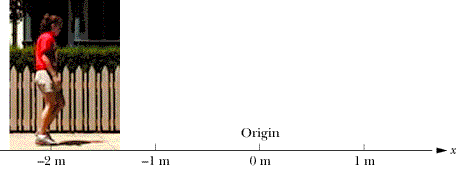
Motion Diagrams: Now that you have learned about position and displacement, it is quite easy to describe the motion of an object using pictures or sketches to chart how position changes over time. Such a representation is called a motion diagram. For example, Fig.  from a point on a sidewalk that we choose as our origin. Figure
 |
| Figure 2-6 A motion diagram of a student standing still with the back of her belt at a horizontal distance of 2.00 m to the left of a spot of the sidewalk designated as the origin. |
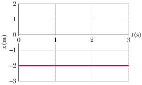
Graphs: Another way to describe how the position of an object changes as time passes is with a graph. In such a graph, the x-component of the object's position, x, can be plotted as a function of time, t. This position-time graph has alternate names such as a graph of x as a function of t, x(t), or x vs. t. For example, Fig.
 |
| Figure 2-8 The graph of the x-component of position for a student who is standing still at x = –2.0 m for at least 3 seconds. |
The graph of no motion shown in Fig.
 | |
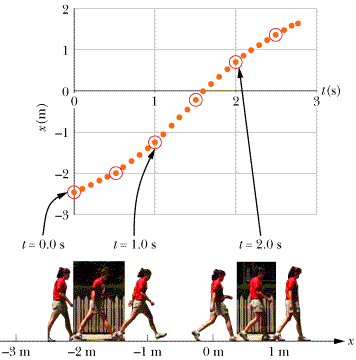
| Figure 2-9 A graph that represents how the position component, x, of the walking student shown in Fig. | |
Although the graph of the student's motion in Fig.
What can motion diagrams and x vs. t graphs tell us about how fast and in what direction something moves along a line? It is clear from an examination of the motion diagram at the bottom of Fig.
 | |
Since time moves forward, t2 > t1, so Dt always has a positive value. Thus, a slope will be positive whenever x2 > x1, so Dx is positive. In this case a straight line connecting the two points on the graph slants upward toward the right when the student is moving along the positive x-direction. On the other hand, if the student were to move “backwards” in the direction along the x axis we chose to call negative, then x2 < x1. In this case, the slope between the two times would be negative and the line connecting the points would slant downward to the right.
Average Velocity
For motion along a straight line, the steepness of the slope in an x vs. t graph over a time interval from t1 to t2 tells us “how fast” a particle moves. The direction of motion is indicated by the sign of the slope (positive or negative). Thus, this slope or ratio  is a special quantity that tells us how fast and in what direction something moves. We haven't given the ratio
  a name yet. We do this to emphasize the fact that the ideas associated with figuring out how fast and in what direction something moves are more important than the names we assign to them. However, it is inconvenient not to have a name.The common name for this ratio is average velocity, which is defined as the ratio of displacement vector
  for the motion of interest to the time interval Dt in which it occurs. This vector can be expressed in equation form as
 | |
 to denote the average of a quantity. Also, we use the special symbol “≡” for equality to emphasize that the term on the left is equal to the term on the right by definition. The time change is a positive scalar quantity because we never need to specify its direction explicitly. In defining
  we are basically multiplying the displacement vector,
  by the scalar (
 ). This action gives us a new vector that points in the same direction as the displacement vector.
Figure
 |
 |
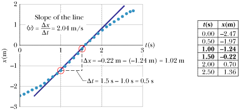
| Figure 2-10 Calculation of the slope of the line that connects the points on the curve at t1 = 1.0 s and t2 = 1.5 s. The xcomponent of the average velocity is given by this slope. |
The x-component of the average velocity along the line of motion,  , is simply the slope of the straight line that connects the point on the curve at the beginning of our chosen interval and the point on the curve at the end of the interval. Since our student is speeding up and slowing down, the values of
  and
and  will in general be different when calculated using other time intervals.
Average Speed
Sometimes we don't care about the direction of an object's motion but simply want to keep track of the distance covered. For instance, we might want to know the total distance a student walks (number of steps times distance covered in each step). Our student could be pacing back and forth wearing out her shoes without having a vector displacement. Similarly, average speed,  , is a different way of describing “how fast” an object moves. Whereas the average velocity involves the particle's displacement
  , which is a vector quantity, the average speed involves the total distance covered (for example, the product of the length of a step and the number of steps the student took), which is independent of direction. So average speed is defined as
 | |
Since neither the total distance traveled nor the time interval over which the travel occurred has an associated direction, average speed does not include direction information. Both the total distance and the time period are always positive, so average speed is always positive too. Thus, an object that moves back and forth along a line can have no vector displacement, so it has zero velocity but a rather high average speed. At other times, while the object is moving in only one direction, the average speed  is the same as the magnitude of the average velocity
  . However, as you can demonstrate in Reading Exercise
  .
.
Instantaneous Velocity and Speed
You have now seen two ways to describe how fast something moves: average velocity and average speed, both of which are measured over a time interval Dt. Clearly, however, something might speed up and slow down during that time interval. For example, in Fig.
Defining an instant and instantaneous velocity is not a trivial task. As we noted in Chapter
For the purpose of finding a velocity at an instant, we can attempt to make the time interval we use in our calculation so small that it has almost zero duration. Of course the displacement we calculate also becomes very small. So instantaneous velocity along a line—like average velocity—is still defined in terms of the ratio of  . But we have this ratio passing to a limit where Dt gets closer and closer to zero. Using standard calculus notation for this limit gives us the following definition:
 | |
In the language of calculus, the INSTANTANEOUS VELOCITY is the rate at which a particle's position vector, |
In passing to the limit the ratio  is not necessarily small, since both the numerator and denominator are getting small together. The first part of this expression,
 |
 |
 and t as a continuous mathematical function such as
  , we can also find the object's instantaneous velocity by taking a derivative with respect to time of the object's position
  . When
  varies continuously as time marches on, we often denote
  as a position function
  to remind us that it varies with time.
Instantaneous speed, which is typically called simply speed, is just the magnitude of the instantaneous velocity vector,  . Speed is a scalar quantity consisting of the velocity value that has been stripped of any indication of the direction the object is moving, either in words or via an algebraic sign. A velocity of (+5 m/s)
 and one of (–5 m/s)
 both have an associated speed of 5 m/s.
| Suppose that you drive 10 mi due east to a store. You suddenly realize that you forgot your money. You turn around and drive the 10 mi due west back to your home and then return to the store. The total trip took 30 min. (a) What is your average velocity for the entire trip? (Set up a coordinate system and express your result in vector notation.) (b) What was your average speed for the entire trip? (c) Discuss why you obtained different values for average velocity and average speed. | ||
| Suppose that you are driving and look down at your speedometer.What does the speedometer tell you—average speed, instantaneous speed, average velocity, instantaneous velocity—or something else? Explain. | ||
|
The following equations give the position component, x(t), along the x axis of a particle's motion in four situations (in each equation, x is in meters, t is in seconds, and t > 0): (1) x = (3 m/s)t – (2 m); (2) x = (–4 m/s2)t2 – (2 m); (3) x = (–4 m/s2)t2; and (4) x = –2 m.
(a) In which situations is the velocity | ||
|
In Touchstone Example | ||
| TOUCHSTONE EXAMPLE 2-2: Out of Gas |
|
You drive a beat-up pickup truck along a straight road for 8.4 km at 70 km/h, at which point the truck runs out of gasoline and stops. Over the next 30 min, you walk another 2.0 km farther along the road to a gasoline station.
(a) What is your overall displacement from the beginning of your drive to your arrival at the station? SOLUTION: Assume, for convenience, that you move in the positive direction along an x axis, from a first position of
Thus, your overall displacement is 10.4 km in the positive direction of the x axis.
| |||||||||||||||||||