2-5

Constant Acceleration: A Special Case

If you watch a small steel ball bobbing up and down at the end of a spring, you will see the velocity changing continuously. But instead of either increasing or decreasing at a steady rate, we have a very nonuniform pattern of motion. First the ball speeds up and slows down moving in one direction, then it turns around and speeds up and then slows down in the other direction, and so on. This is an example of a nonconstant acceleration that keeps changing in time.

Although there are many examples of nonconstant accelerations, we also observe a surprising number of examples of constant or nearly constant acceleration. As we already discussed, Galileo discovered that if we choose to define acceleration in terms of the ratio , then a falling ball or a ball tossed into the air that slows down, turns around, and speeds up again is always increasing its velocity in a downward direction at the same rate—provided the ball is moving slowly enough that air drag is negligible.

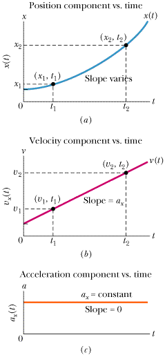
There are many other common motions that involve constant accelerations. Suppose you measure the times and corresponding positions for an object that you suspect has a constant acceleration. If you then calculate the velocities and accelerations of the object and make graphs of them, the graphs will resemble those in Fig. 2-14. Some examples of motions that yield similar graphs to those shown in Fig. 2-14 include: a car that you accelerate as soon as a traffic light turns green; the same car when you apply its brakes steadily to bring it to a smooth stop; an airplane when first taking off or when completing a smooth landing; or a dolphin that speeds up suddenly after being startled.

Figure 2-14 (a) The position component x(t) of a particle moving with constant acceleration. (b) Its velocity component vx(t), given at each point by the slope of the curve in (a). (c) Its (constant) component of acceleration, ax, equal to the (constant) slope of vx(t).

Derivation of the Kinematic Equations

Because constant accelerations are common, it is useful to derive a special set of kinematic equations to describe the motion of any object that is moving along a line with a constant acceleration. We can use the definitions of acceleration and velocity and an assumption about average velocity to derive the kinematic equations. These equations allow us to use known values of the vector components describing positions, velocities, and accelerations, along with time intervals to predict the motions of constantly accelerated objects.

Let's start the derivation by noting that when the acceleration is constant, the average and instantaneous accelerations are equal. As usual we place our x axis along the line of the motion. We can now use vector notation to write

(2-11)

(2-12)

This expression allows us to derive the kinematic equations in terms of the vector components needed to construct the actual one-dimensional velocity and acceleration vectors. The subscripts 1 and 2 in most of the equations in this chapter, including Eq. 2-12, refer to initial and final times, positions, and velocities.

If we solve Eq. 2-12 for v_2x, then the x-component of velocity at time t₂ is

(2-13)

This equation is the first of two primary equations that we will derive for use in analyzing motions involving constant acceleration. Before we move on, we should think carefully about what the expression t₂ – t₁ represents in this equation: It represents the time interval in which we are tracking the motion.

In a manner similar to what we have done above, we can rewrite Eq. 2-4, the expression for the average velocity along the x axis,

Hence, the x-component of the average velocity is given by

(2-14)

In this equation x₁ is the x-component of the position of the particle at t = t₁ and is the component along the x axis of average velocity between t = t₁ and a later time t = t₂. Note that unless the velocity is constant, the average velocity component along the x axis, , is not equal to the instantaneous velocity component, v_x.

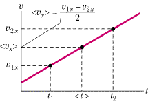
However, we do have a plausible alternative for expressing the average velocity component in the special case when the acceleration is constant. Figure 2-15 depicts the fact that velocity increases in a linear fashion over time for a constant acceleration. It seems reasonable to assume that the component along the x axis of the average velocity over any time interval is the average of the components for the instantaneous velocity at the beginning of the interval, v_1x, and the instantaneous velocity component at the end of the interval, v_2x. So we expect that when a velocity increases linearly, the average velocity component over a given time interval will be

(2-15)

Using Eq. 2-13, we can substitute v_1x + a_x(t₂ – t₁) for v_2x to get

(2-16)

Finally, substituting this equation into Eq. 2-14 yields

(2-17)  or

Figure 2-15 When the acceleration is constant, then we assume (without rigorous proof) that the average velocity component in a time interval is the average of the velocity components at the beginning and end of the interval.

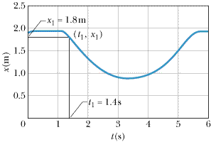
This is our second primary equation describing motion with constant acceleration. Figures 2-14a and 2-16 show plots of Eq. 2-17.

Figure 2-16 A fan on a low-friction cart is turned on at about 1.2 s but isn't thrusting fully until t1 = 1.4 s. Data for the graph were collected with a computer data acquisition system outfitted with an ultrasonic motion detector. Between 1.4 s and about 5.4 s the cart appears to be undergoing a constant acceleration as it slows down, turns around, and speeds up again. Thus, the constant acceleration kinematic equations can be used to describe its motion but only during motion within that time interval.Thus, we can set t1 to 1.4 s and x1 to 1.8 m.

These two equations are very useful in the calculation of unknown quantities that can be used to characterize constantly accelerated motion. There are five or six quantities contained in our primary equations (Eqs. 2-13 and 2-17). The simplest kinematic calculations involve situations in which all but one of the quantities is known in one of the primary equations. In more complex situations, both equations are needed. Typically for a complex situation, we need to calculate more than one unknown. To do this, we find the first unknown using one of the primary equations and use the result in the other equations to find the second unknown. This method is illustrated in the next section and in Touchstone Examples 2-4 and 2-6.

The primary equations above, v_2x = v_1x + a_x(t₂ – t₁) = v_1x + a_xDt (Eq. 2-13), and (Eq. 2-17), are derived directly from the definitions of velocity and acceleration, with the condition that the acceleration is constant. These two equations can be combined in three ways to yield three additional equations. For example, solving for v_1x in v_2x = v_1x + a_x(t₂ – t₁) and substituting the result into gives us

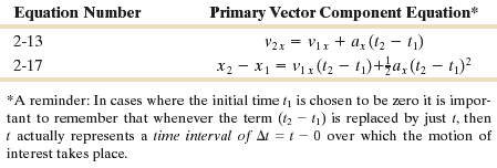
We recommend that you learn the two primary equations and use them to derive other equations as needed. Then you will not need to remember so much. Table 2-1 lists our two primary equations. Note that a really nice alternative to using the two equations in Table 2-1 is to use the first of the equations (Eq. 2-13) along with the expression for the average velocity component in Eq. 2-15,

TABLE 2-1

Equations of Motion with Constant Acceleration

Analyzing the Niagara Falls Plunge

At the beginning of this chapter we asked questions about the motion of the steel chamber holding Dave Munday as he plunged into the water after falling 48 m from the top of Niagara Falls. How long did the fall take? That is, what is Dt? How fast was the chamber moving when it hit the water? (What is ) As you will learn in Chapter 3, if no significant air drag is present, objects near the surface of the Earth fall at a constant acceleration of magnitude . Thus, the kinematic equations can be used to calculate the time of fall and the impact speed.

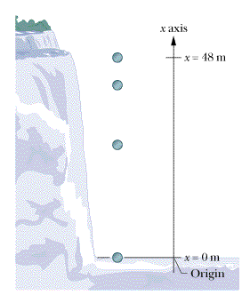
Let's start by defining our coordinate system.We will take the x axis to be a vertical or up-down axis that is aligned with the downward path of the steel chamber. We place the origin at the bottom of the falls and define up to be positive as shown in Fig. 2-17. (Later when considering motions in two and three dimensions, we will often denote vertical axes as y axes and horizontal axes as x axes, but these changes in symbols will not affect the results of calculations.)

Figure 2-17 A coordinate system chosen to analyze the fall of a steel chamber holding a man who falls 48 m from the top to the bottom of Niagara Falls.

We know that the value of the vertical displacement is given by

Next we can use the time interval of the fall in the other primary kinematic equation, Eq. 2-13, to find the velocity at impact.This gives a component of impact velocity at the end of the fall of

The minus sign indicates that the impact velocity component is negative and is, therefore, in the downward direction. In vector notation, the velocity is thus . Note that this is a speed of about 69 mi/hr. Since the time interval was put into the calculation of velocity of impact as an intermediate value, we retained an extra significant figure to use in the next calculation.

READING EXERCISE 2-9:		The following equations give the x-component of position x(t) of a particle in meters (denoted m) as a function of time in seconds for four situations: (1) x = (3 m/s)t – 4 m; (2) x = (– 5 m/s3)t3 + (4 m/s)t + 6 m; (3) x = (2 m/s2)t2 – (4 m/s)t; (4) x = (5 m/s2)t2 – 3 m. To which of these situations do the equations of Table 2-1 apply? Explain.

TOUCHSTONE EXAMPLE 2-4: Slowing Down

Spotting a police car, you brake your Porsche from a speed of 100 km/h to a speed of 80.0 km/h during a displacement of 88.0 m, at a constant acceleration. (a) What is that acceleration? SOLUTION: Assume that the motion is along the positive direction of an x axis. For simplicity, let us take the beginning of the braking to be at time t1 = 0, at position x1. The Key Idea here is that, with the acceleration constant, we can relate the car's acceleration to its velocity and displacement via the basic constant acceleration equations (Eqs. 2-13 and 2-17). The initial velocity is v1x = 100 km/h = 27.78 m/s, the displacement is x2 – x1 = 88.0 m, and the velocity at the end of that displacement is v2x = 80.0 km/h = 22.22 m/s. However, we do not know the acceleration ax and time t2, which appear in both basic equations, so we must solve those equations simultaneously. To eliminate the unknown t2, we use Eq. 2-13 to write  (2-18)  and then we substitute this expression into Eq. 2-17 to write Solving for ax and substituting known data then yields  (Answer)  .   (b) How much time is required for the given decrease in speed? SOLUTION: Now that we know ax, we can use Eq. 2-18 to solve for t2:  (Answer)  If you are initially speeding and trying to slow to the speed limit, there is plenty of time for the police officer to measure your excess speed. You can use one of the alternate equations for motion with a constant acceleration, Eq. 2-15, to check this result.The Key Idea here is that the distance traveled is just the product of the average velocity and the elapsed time, when the acceleration is constant. The Porsche traveled 88.0 m while it slowed from 100 km/h down to 80 km/h. Thus its average velocity while it covered the 88.0 m was so the time it took to slow down was just  (Answer)  which still isn't enough time to avoid that speeding ticket!

TOUCHSTONE EXAMPLE 2-5: Motion Data

Suppose that you gave a box sitting on a carpeted floor a push and then recorded its position three times per second as it slid to a stop. The table gives the results of such a measurement. Let's analyze the position vs. time data for the box sliding on the carpet and use curve fitting and calculus to obtain the velocity measurements. We will use Excel spreadsheet software to perform our analysis, but other computer- or calculator-based fitting or modeling software can be used. (a) Draw a graph of the x vs. t data and discuss whether the relationship appears to be linear or not. SOLUTION: The Key Idea here is that the relationship between two variables is linear if the graph of the data points lie more or less along a straight line.There are many ways to graph the data for examination: by hand, with a graphing calculator, with a spreadsheet graphing routine, or with other graphing software such as Data Studio (available from PASCO scientific) or Graphical Analysis (available from Vernier Software and Technology). The graph in Fig. 2-18 that shows a curve and so the relationship between position, x, and time is not linear. 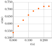Figure 2-18 Solution to Touchstone Example 2-5(a). A graph of position versus time for a box sliding across a carpet. .   (b) Draw a motion diagram of the box as it comes to rest on the carpet. SOLUTION: The Key Idea here is to use the data to sketch the position along a line at equal time intervals. In Fig. 2-19, the black circles represent the location of the rear of the box at intervals of 1/30 of a second. Figure 2-19 Solution to Touchstone Example 2-5(b). A motion diagram for a box sliding across a carpet. .   (c) Is the acceleration constant? If so, what is its component along the x axis? SOLUTION: The Key Idea here is to explore whether or not the relationship between position and time of the box as it slides to a stop can be described with a quadratic (parabolic) function of time as described in Eq. 2-17. This can be done by entering the data that are given into a spreadsheet or graphing calculator and either doing a quadratic model or a fit to the data.The outcome of a quadratic model is shown in Fig. 2-20. The x-model column contains the results of calculating x using the equation for each of the times in the first column using the initial position, velocity and acceleration data shown in the boxes. The line shows the model data. If the kinematic equation fits the data, then we can conclude that the acceleration component is a constant given by ax = –6.6 m/s2. Thus the acceleration is in the negative y direction. Figure 2-20 Solution to Touchstone Example (c). Data and a graph of position as function of time for a box sliding over carpet. Actual data is compared to a model of what is expected from Eq. 2-17 (assumed constant acceleration).The value of acceleration which produced the best match between the model and actual data is –6.6 m/s2.

TOUCHSTONE EXAMPLE 2-6: Distance Covered

Figure 2-21b shows a graph of a person riding on a low-friction cart being pulled along with a bungee cord as shown in Fig. 2-21a. Use information from the two graphs and the kinematic equations to determine approximately how far the student moved in the time interval between 1.1 s and 2.0 s. Figure 2-21 (a) A person riding on a low-friction cart is pulled by another person who exerts a constant force along a straight line by keeping the length of a bungee cord constant. (b) These graphs show velocity and acceleration components vs. time for a rider on a cart. For the first 0.5 s (region A) the cart is at rest. Between 0.5 s and 1.1 s (region B) the cord is beginning to stretch. Between 1.1 s and 2.0 s (region C) a constant force is acting and the acceleration is also constant. SOLUTION: The Key Idea is that the initial velocity can be determined from the velocity vs. time graph on the left and the acceleration during the time interval can be determined from the acceleration vs. time graph on the right (or by finding the slope of the velocity vs. time graph on the left during the time interval). Note that the velocity at t1 = 1.1 s is given by v1x ≈ 0.4 m/s. The acceleration during the time interval of interest is given by a1x ≈ 0.4 m/s2. Since the acceleration is constant over the time interval of interest, we can use the data in Eq. 2-17 to get  (Answer)  Half a meter is not very far!

Copyright © 2000-2003 by John Wiley & Sons, Inc. or related companies. All rights reserved.