| 3.9 |
Linear Approximation and the Derivative
|
The Tangent Line Approximation
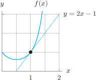
When we zoom in on the graph of a differentiable function, it looks like a straight line. In fact, the graph is not exactly
a straight line when we zoom in; however, its deviation from straightness is so small that it can't be detected by the naked
eye. Let's examine what this means. The straight line that we think we see when we zoom in on the graph of  at
at  has slope equal to the derivative,
  , so the equation is
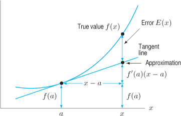
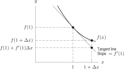
The fact that the graph looks like a line means that  is a good approximation to . (See Figure 3.40.) This suggests the following definition:
It can be shown that the tangent line approximation is the best linear approximation to  near
near  . See Problem 43.
at has slope equal to the derivative, , so the equation is
|
 is a good approximation to . (See Figure 3.40.) This suggests the following definition:
|
 is called the
  near . See Problem 43.
|
|||
|
|
 near
near 
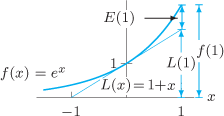
 , then
  , so
, so  and
and  , and the approximation is

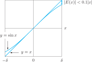
 . If we zoom in on the graphs of the functions
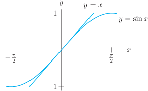

|
 near
near  , then
  and, by the chain rule,
  , so
, so  . Thus

 and
and  near the origin, we won't be able to tell them apart.
Estimating the Error in the Approximation
Let us look at the error,  , which is the difference between and the local linearization. (Look back at Figure 3.40.) The fact that the graph of looks like a line as we zoom in means that not only is small for
  near , but also that is small relative to
  . To demonstrate this, we prove the following theorem about the ratio
  .
.
, which is the difference between and the local linearization. (Look back at Figure 3.40.) The fact that the graph of looks like a line as we zoom in means that not only is small for near , but also that is small relative to . To demonstrate this, we prove the following theorem about the ratio .
|

|

 and using the definition of the derivative, we see that

Theorem 3.6 says that approaches 0 faster than . For the function in Example 3, we see that  for constant
  if is near .
approaches 0 faster than . For the function in Example 3, we see that for constant if is near .
|
 for
for  suggest about
  ?
?
 . Estimate the value of
  .
.
 , and
, and  . Thus,
  and
and  , so the tangent line approximation for

 .
.
 , then
  . Thus we make Table
  . Since the values are all approximately 6, we guess that
  and
and  .
.
 , our value of
 The relationship between and  that appears in Example 1 holds more generally. If satisfies certain conditions, it can be shown that the error in the tangent line approximation behaves near as
This is part of a general pattern for obtaining higher-order approximations called Taylor polynomials, which are studied in
Chapter 10.
and that appears in Example 1 holds more generally. If satisfies certain conditions, it can be shown that the error in the tangent line approximation behaves near as
|
Why Differentiability Makes a Graph Look Straight
We use the properties of the error to understand why differentiability makes a graph look straight when we zoom in.
to understand why differentiability makes a graph look straight when we zoom in.
|
 for all

 , then the definition of limit guarantees that there is a
  such that
 , we have
  , so
, so

 and its linear approximation
  , showing a window in which the magnitude of the error,
  , is less than
  for all
  in the window
We can generalize from this example to explain why differentiability makes the graph of look straight when viewed over a small graphing window. Suppose is differentiable at . Then we know  . So, for any
  , we can find a δ small enough so that
So, for any in the interval  , we have
Thus, the error, , is less than ε times  , the distance between and . So, as we zoom in on the graph by choosing smaller ε, the deviation,
  , of from its tangent line shrinks, even relative to the scale on the
  . So, zooming makes a differentiable function look straight.
look straight when viewed over a small graphing window. Suppose is differentiable at . Then we know . So, for any , we can find a δ small enough so that
|
 in the interval , we have
|
 , is less than ε times , the distance between and . So, as we zoom in on the graph by choosing smaller ε, the deviation, , of from its tangent line shrinks, even relative to the scale on the . So, zooming makes a differentiable function look straight.
Exercises and Problems for Section 3.9
Exercises
| 1. |
Find the tangent line approximation for
 near near  . .
  |
 , the chain rule gives
  , so
, so  . Therefore the tangent line approximation of
  near
near 

 . (See figure
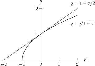
| 2. |
What is the tangent line approximation to
 near ? near ?
|
| 3. |
Find the tangent line approximation to
 near near  . .
|

| 4. |
Find the local linearization of
 near . near .
|
| 5. |
What is the local linearization of
 near ? near ?
|

 , we get a tangent line approximation of
  which becomes
  . Thus, our local linearization of
  near
near  .
.
| 6. |
Show that
 is the tangent line approximation to is the tangent line approximation to  near . near .
|
| 7. |
Show that
 near . near .
|
| 8. |
Local linearization gives values too small for the function
 and too large for the function and too large for the function  . Draw pictures to explain why. . Draw pictures to explain why.
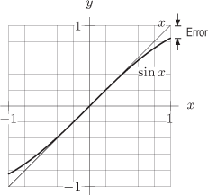
|
| 9. |
Using a graph like Figure 3.41, estimate to one decimal place the magnitude of the error in approximating sin
by for  . Is the approximation an over- or an underestimate? . Is the approximation an over- or an underestimate?
|


 . The magnitude of the error can be read off the graph as less than 0.2 or estimated as

| 10. |
For
near 0, local linearization gives
.
|

Problems
| 11. |
|
 , to
, to 
 for
for 
 or
or  , and why.
| 12. |
|
 at
at  .
.
 .
.
| 13. |
|
 .
.
 .
.

 , we have
  , so
, so  , and the local linearization is
  .
.
 , the tangent line approximation to
 | 14. |
|
 is the local linearization of
  near
near | 15. |
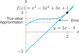
Figure 3.43 shows
and its local linearization at . What is the value of ? Of  ? Is the approximation an under- or overestimate? Use the linearization to approximate the value of ? Is the approximation an under- or overestimate? Use the linearization to approximate the value of  . .
|


In Problems 16-17, the equation has a solution near . By replacing the left side of the equation by its linearization, find an approximate value for the solution.
. By replacing the left side of the equation by its linearization, find an approximate value for the solution.
| 16. |
 |
| 17. |
 |
 , so
, so  . Thus
  so
so


 .
.
| 18. |
|
 and
and  , estimate
  .
.
 for all
 | 19. |
|
 by its linearization near 0. Solve the new equation to get an approximate solution to the original equation.
| 20. |
The speed of sound in dry air is
 is the temperature in is the temperature in  . Find a linear function that approximates the speed of sound for temperatures near . Find a linear function that approximates the speed of sound for temperatures near  . .
|
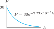
| 21. |
Air pressure at sea level is 30 inches of mercury. At an altitude of
 feet above sea level, the air pressure, feet above sea level, the air pressure,  , in inches of mercury, is given by , in inches of mercury, is given by
|
 .
.
 , so the equation of the tangent line is

 , so
, so


 intercepts of 30, and the slopes are almost the same
  . The rule of thumb calculates values of
  ). Thus, the rule of thumb values are slightly smaller.
| 22. |
On October 7, 2010, the Wall Street Journal8 reported that Android cell phone users had increased to 10.9 million by the end of August 2010 from 866,000 a year earlier.
During the same period, iPhone users increased to 13.5 million, up from 7.8 million a year earlier. Let
 be the number of Android users, in millions, at time t in years since the end of August 2009. Let be the number of Android users, in millions, at time t in years since the end of August 2009. Let  be the number of iPhone users in millions. be the number of iPhone users in millions.
|
 . Give units.
 . Give units.
| 23. |
Writing
 for the acceleration due to gravity, the period, , of a pendulum of length for the acceleration due to gravity, the period, , of a pendulum of length  is given by is given by
|

 , the change in the period,
  , is given by

| 24. |
Suppose now the length of the pendulum in Problem 23 remains constant, but that the acceleration due to gravity changes.
|
 , the change in
 | 25. |
Suppose
has a continuous positive second derivative for all . Which is larger,  or or  ? Explain. ? Explain.
|
 positive, but the result is also true if
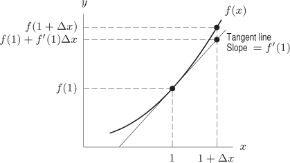
| 26. |
Suppose
 is a differentiable decreasing function for all . In each of the following pairs, which number is the larger? Give a reason for your answer. is a differentiable decreasing function for all . In each of the following pairs, which number is the larger? Give a reason for your answer.
|
 and
and 
 and 0
and 0
 and
and 
Problems 27-29 investigate the motion of a projectile shot from a cannon. The fixed parameters are the acceleration of gravity,
 , and the muzzle velocity,
  , at which the projectile leaves the cannon. The angle
  , in degrees, between the muzzle of the cannon and the ground can vary.
, and the muzzle velocity, , at which the projectile leaves the cannon. The angle , in degrees, between the muzzle of the cannon and the ground can vary.
| 27. |
The range of the projectile is
|
 .
.

 .
.

 .
.


| 28. |
The time that the projectile stays in the air is
|
| 29. |
At its highest point the projectile reaches a peak altitude given by
|

 meters

 , near


 . The linear approximation gives

In Problems 30-32, find the local linearization of  near 0 and use this to approximate the value of .
near 0 and use this to approximate the value of .
| 30. |
 |
| 31. |
 |

| 32. |
 |
In Problems 33-37, find a formula for the error in the tangent line approximation to the function near . Using a table of values for near , find a value of such that  . Check that, approximately,
  and that
  .
.
in the tangent line approximation to the function near . Using a table of values for near , find a value of such that . Check that, approximately, and that .
| 33. |
 , ,  |
 and
and  . Thus
 near
near 
 , so
, so
 using
using  and expanding:


 is small, so we ignore powers of
 | 34. |
 , ,  |
| 35. |
 , , |
| 36. |
 |
| 37. |
 , , |
 and
and  . Thus


 and
and
 , so
, so
| 38. |
Multiply the local linearization of
near by itself to obtain an approximation for  . Compare this with the actual local linearization of . Explain why these two approximations are consistent, and discuss which one is more accurate. . Compare this with the actual local linearization of . Explain why these two approximations are consistent, and discuss which one is more accurate.
|
| 39. |
|
 is the local linearization of
  near
near 
 is at
is at | 40. |
From the local linearizations of
and  near , write down the local linearization of the function near , write down the local linearization of the function  . From this result, write down the derivative of . From this result, write down the derivative of  at . Using this technique, write down the derivative of at . Using this technique, write down the derivative of  at . at .
|
| 41. |
Use local linearization to derive the product rule,
 |

 .]
.]
 ,
,  , and
, and  . Therefore

 . (This implies that
  .)
.)
 and
and  cancel out. All the remaining terms on the right, with the exception of the second and third terms, go to zero as
  . Thus, we have

| 42. |
Derive the chain rule using local linearization.
|
 , using
  .]
.]
| 43. |
Consider a function
and a point . Suppose there is a number  such that the linear function such that the linear function
. By good approximation, we mean that
 is the approximation error defined by is the approximation error defined by
is differentiable at and that  . Thus the tangent line approximation is the only good linear approximation. . Thus the tangent line approximation is the only good linear approximation.
|

| 44. |
Consider the graph of
near . Find an interval around with the property that throughout any smaller interval, the graph of never differs from its local linearization at by more than  . .
|
Strengthen Your Understanding
In Problems 45-46, explain what is wrong with the statement.
| 45. |
To approximate
 , we can always use the linear approximation , we can always use the linear approximation  . .
|
 is the linear approximation for
  (instead of 2.718). For
  .
.
| 46. |
The linear approximation for
 near near  is an underestimate for the function is an underestimate for the function  for all , for all ,  . .
|
In Problems 47-49, give an example of:
| 47. |
Two different functions that have the same linear approximation near
.
|
| 48. |
A non-polynomial function that has the tangent line approximation
 near . near .
|
| 49. |
A function that does not have a linear approximation at
 . .
|

 , is given by
  . Since
  does not have a derivative at
  this function does not have a linear approximation for
  . Other answers are possible.
| 50. |
Let
be a differentiable function and let be the linear function  for some constant . Decide whether the following statements are true or false for all constants . Explain your answer. for some constant . Decide whether the following statements are true or false for all constants . Explain your answer.
|
 , then