Average Velocity and Average Speed

2-4 Average Velocity and Average Speed

A compact way to describe position is with a graph of position x plotted as a function of time t—a graph of x(t). (The notation x(t) represents a function x of t, not the product x times t.) As a simple example, Figure 2-2 shows the position function x(t) for a stationary armadillo (which we treat as a particle) over a 7 s time interval. The animal's position stays at x = -2 m.

Fig. 2-2 The graph of x(t) for an armadillo that is stationary at x = -2 m. The value of x is -2 m for all times t.

Figure 2-3a is more interesting, because it involves motion. The armadillo is apparently first noticed at t = 0 when it is at the position x = -5 m. It moves toward x = 0, passes through that point at t = 3 s, and then moves on to increasingly larger positive values of x. Figure 2-3b depicts the straight-line motion of the armadillo and is something like what you would see. The graph in Figure 2-3a is more abstract and quite unlike what you would see, but it is richer in information. It also reveals how fast the armadillo moves.

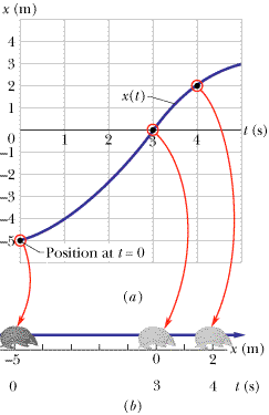Fig. 2-3 (a) The graph of x(t) for a moving armadillo. (b) The path associated with the graph. The scale below the x axis shows the times at which the armadillo reaches various x values.

Actually, several quantities are associated with the phrase “how fast.” One of them is the average velocity v_avg, which is the ratio of the displacement Dx that occurs during a particular time interval Dt to that interval:

(2-2)

The notation means that the position is x₁ at time t₁ and then x₂ at time t₂. A common unit for v_avg is the meter per second (m/s). You may see other units in the problems, but they are always in the form of length/time.

On a graph of x versus t, v_avg is the slope of the straight line that connects two particular points on the x(t) curve: one is the point that corresponds to x₂ and t₂, and the other is the point that corresponds to x₁ and t₁. Like displacement, v_avg has both magnitude and direction (it is another vector quantity). Its magnitude is the magnitude of the line's slope. A positive v_avg (and slope) tells us that the line slants upward to the right; a negative v_avg (and slope) tells us that the line slants downward to the right. The average velocity v_avg always has the same sign as the displacement Dx because Dt in Equation 2-2 is always positive.

Figure 2-4 shows how to find v_avg in Figure 2-3 for the time interval t = 1 s to t = 4 s. We draw the straight line that connects the point on the position curve at the beginning of the interval and the point on the curve at the end of the interval. Then we find the slope Dx/Dt of the straight line. For the given time interval, the average velocity is

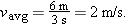Fig. 2-4 Calculation of the average velocity between t = 1 s and t = 4 s as the slope of the line that connects the points on the x(t) curve representing those times.

Average speed s_avg is a different way of describing “how fast” a particle moves. Whereas the average velocity involves the particle's displacement Dx, the average speed involves the total distance covered (for example, the number of meters moved), independent of direction; that is,

(2-3)

Because average speed does not include direction, it lacks any algebraic sign. Sometimes s_avg is the same (except for the absence of a sign) as v_avg. However, as is demonstrated in Sample Problem 2-1, when an object doubles back on its path, the two can be quite different.

Sample Problem 2-1

You drive a beat-up pickup truck along a straight road for 8.4 km at 70 km/h, at which point the truck runs out of gasoline and stops. Over the next 30 min, you walk another 2.0 km farther along the road to a gasoline station.

(a) What is your overall displacement from the beginning of your drive to your arrival at the station?

Solution: Assume, for convenience, that you move in the positive direction of an x axis, from a first position of x₁ = 0 to a second position of x₂ at the station. That second position must be at x₂ = 8.4 km + 2.0 km = 10.4 km. Then the Key Idea here is that your displacement Dx along the x axis is the second position minus the first position. From Equation 2-1, we have

(Answer)

Thus, your overall displacement is 10.4 km in the positive direction of the x axis.

(b) What is the time interval Dt from the beginning of your drive to your arrival at the station?

Solution: We already know the walking time interval Dt_wlk (= 0.50 h), but we lack the driving time interval Dt_dr. However, we know that for the drive the displacement Dx_dr is 8.4 km and the average velocity v_avg,dr is 70 km/h. A Key Idea to use here comes from Equation 2-2: This average velocity is the ratio of the displacement for the drive to the time interval for the drive:

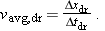Rearranging and substituting data then give us

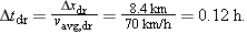So,

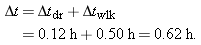(Answer)

(c) What is your average velocity v_avg from the beginning of your drive to your arrival at the station? Find it both numerically and graphically.

Solution: The Key Idea here again comes from Equation 2-2: v_avg for the entire trip is the ratio of the displacement of 10.4 km for the entire trip to the time interval of 0.62 h for the entire trip. Here we find

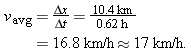(Answer)

To find v_avg graphically, first we graph the function x(t) as shown in Figure 2-5, where the beginning and arrival points on the graph are the origin and the point labeled as “Station.” The Key Idea here is that your average velocity is the slope of the straight line connecting those points; that is, v_avg is the ratio of the rise (Dx = 10.4 km) to the run (Dt = 0.62 h), which gives us v_avg = 16.8 km/h.

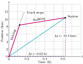Fig. 2-5 The lines marked “Driving” and “Walking” are the position-time plots for the driving and walking stages. (The plot for the walking stage assumes a constant rate of walking.) The slope of the straight line joining the origin and the point labeled “Station” is the average velocity for the trip, from the beginning to the station.

(d) Suppose that to pump the gasoline, pay for it, and walk back to the truck takes you another 45 min. What is your average speed from the beginning of your drive to your return to the truck with the gasoline?

Solution: The Key Idea here is that your average speed is the ratio of the total distance you move to the total time interval you take to make that move. The total distance is 8.4 km + 2.0 km + 2.0 km = 12.4 km. The total time interval is 0.12 h + 0.50 h + 0.75 h = 1.37 h. Thus, Equation 2-3 gives us

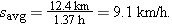(Answer)

	CHECKPOINT 2 In this sample problem, suppose that right after refueling the truck, you drive back to x₁ at 35 km/h. What is your average velocity for your entire trip?

PROBLEM-SOLVING TACTICS

TACTIC 1: Do You Understand the Problem?

For beginning problem solvers, no difficulty is more common than simply not understanding the problem. The best test of understanding is this: Can you explain the problem?

Write down the given data, with units, using the symbols of the chapter. (In Sample Problem 2-1, the given data allow you to find your net displacement Dx in part (a) and the corresponding time interval Dt in part (b).) Identify the unknown and its symbol. (In the sample problem, the unknown in part (c) is your average velocity v_avg.) Then find the connection between the unknown and the data. (The connection is provided by Equation 2-2, the definition of average velocity.)

TACTIC 2: Are the Units OK?

Be sure to use a consistent set of units when putting numbers into the equations. In Sample Problem 2-1, the logical units in terms of the given data are kilometers for distances, hours for time intervals, and kilometers per hour for velocities. You may sometimes need to convert units.

TACTIC 3: Is Your Answer Reasonable?

Does your answer make sense, or is it far too large or far too small? Is the sign correct? Are the units appropriate? In part (c) of Sample Problem 2-1, for example, the correct answer is 17 km/h. If you find 0.00017 km/h, -17 km/h, 17 km/s, or 17000 km/h, you should realize at once that you have done something wrong. The error may lie in your method, in your algebra, or in your keystroking of numbers on a calculator.

TACTIC 4: Reading a Graph

Figure 2-2, Figure 2-3, Figure 2-4 and Figure 2-5 are graphs you should be able to read easily. In each graph, the variable on the horizontal axis is the time t, with the direction of increasing time to the right. In each, the variable on the vertical axis is the position x of the moving particle with respect to the origin, with the positive direction of x upward. Always note the units (seconds or minutes; meters or kilometers) in which the variables are expressed.

2.9 Interactive Learningware

2.11 Interactive Learningware