2-7  Constant Acceleration: A Special Case

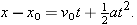
In many types of motion, the acceleration is either constant or approximately so. For example, you might accelerate a car at an approximately constant rate when a traffic light turns from red to green. Then graphs of your position, velocity, and acceleration would resemble those in Figure 2-8. (Note that a(t) in Figure 2-8 is constant, which requires that v(t) in Figure 2-8 have a constant slope.) Later when you brake the car to a stop, the acceleration (or deceleration in common language) might also be approximately constant.

Fig. 2-8 (a) The position x(t) of a particle moving with constant acceleration. (b) Its velocity v(t), given at each point by the slope of the curve of x(t). (c) Its (constant) acceleration, equal to the (constant) slope of the curve of v(t).

One-Dimensional Constant Acceleration

Such cases are so common that a special set of equations has been derived for dealing with them. One approach to the derivation of these equations is given in this section. A second approach is given in the next section. Throughout both sections and later when you work on the homework problems, keep in mind that these equations are valid only for constant acceleration (or situations in which you can approximate the acceleration as being constant).

When the acceleration is constant, the average acceleration and instantaneous acceleration are equal and we can write Equation 2-7, with some changes in notation, as

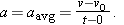Here v₀ is the velocity at time t = 0 and v is the velocity at any later time t. We can recast this equation as

(2-11)

As a check, note that this equation reduces to v = v₀ for t = 0, as it must. As a further check, take the derivative of Equation 2-11. Doing so yields dv/dt = a, which is the definition of a. Figure 2-8c shows a plot of Equation 2-11, the v(t) function; the function is linear and thus the plot is a straight line.

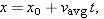
In a similar manner, we can rewrite Equation 2-2 (with a few changes in notation) as

and then as

(2-12)

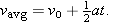
in which x₀ is the position of the particle at t = 0 and v_avg is the average velocity between t = 0 and a later time t.

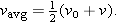
For the linear velocity function in Equation 2-11, the average velocity over any time interval (say, from t = 0 to a later time t) is the average of the velocity at the beginning of the interval (= v₀) and the velocity at the end of the interval (= v). For the interval from t = 0 to the later time t then, the average velocity is

(2-13)

Substituting the right side of Equation 2-11 for v yields, after a little rearrangement,

(2-14)

Finally, substituting Equation 2-14 into Equation 2-12 yields

(2-15)

As a check, note that putting t = 0 yields x = x₀, as it must. As a further check, taking the derivative of Equation 2-15 yields Equation 2-11, again as it must. Figure 2-8 shows a plot of Equation 2-15; the function is quadratic and thus the plot is curved.

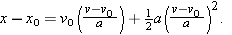
Equation 2-11 and Equation 2-15 are the basic equations for constant acceleration; they can be used to solve any constant acceleration problem in this book. However, we can derive other equations that might prove useful in certain specific situations. First, note that as many as five quantities can possibly be involved in any problem about constant acceleration—namely, x - x₀, v, t, a, and v₀. Usually, one of these quantities is not involved in the problem, either as a given or as an unknown. We are then presented with three of the remaining quantities and asked to find the fourth.

Equation 2-11 and Equation 2-15 each contain four of these quantities, but not the same four. In Equation 2-11, the “missing ingredient” is the displacement x - x₀. In Equation 2-15, it is the velocity v. These two equations can also be combined in three ways to yield three additional equations, each of which involves a different “missing variable.” First, we can eliminate t to obtain

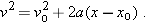(2-16)

This equation is useful if we do not know t and are not required to find it. Second, we can eliminate the acceleration a between Equation 2-11 and Equation 2-15 to produce an equation in which a does not appear:

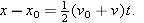(2-17)

Finally, we can eliminate v₀, obtaining

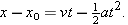(2-18)

Note the subtle difference between this equation and Equation 2-15. One involves the initial velocity v₀; the other involves the velocity v at time t.

Table 2-1 lists the basic constant acceleration equations (Equation 2-11 and Equation 2-15) as well as the specialized equations that we have derived. To solve a simple constant acceleration problem, you can usually use an equation from this list (if you have the list with you). Choose an equation for which the only unknown variable is the variable requested in the problem. A simpler plan is to remember only Equation 2-11 and Equation 2-15, and then solve them as simultaneous equations whenever needed. An example is given in Sample Problem 2-5.

Constant velocity versus constant acceleration

TABLE 2-1

Equations for Motion with Constant Acceleration2

	CHECKPOINT 5    The following equations give the position x(t) of a particle in four situations: (1) x = 3t - 4; (2) x = -5t3 + 4t2 + 6; (3) x = 2/t2 - 4/t; (4) x = 5t2 - 3. To which of these situations do the equations of Table 2-1 apply?

Sample Problem 2-5

Spotting a police car, you brake a Porsche from a speed of 100 km/h to a speed of 80.0 km/h during a displacement of 88.0 m, at a constant acceleration.

(a)  What is that acceleration?

Solution: Assume that the motion is along the positive direction of an x axis. For simplicity, let us take the beginning of the braking to be at time t = 0, at position x₀. The Key Idea here is that, with the acceleration constant, we can relate the car's acceleration to its velocity and displacement via the basic constant acceleration equations (Equation 2-11 and Equation 2-15). The initial velocity is v₀ = 100 km/h = 27.78 m/s, the displacement is x - x₀ = 88.0 m, and the velocity at the end of that displacement is v = 80.0 km/h = 22.22 m/s. However, we do not know the acceleration a and time t, which appear in both basic equations. So, we must solve those equations simultaneously.

To eliminate the unknown t, we use Equation 2-11 to write

(2-19)

and then we substitute this expression into Equation 2-15 to write

Solving for a and substituting known data then yield

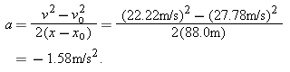(Answer)

Note that we could have used Equation 2-16 instead to solve for a because the unknown t is the missing variable in that equation.

(b)  How much time is required for the given decrease in speed?

Solution: Now that we know a, we can use Equation 2-19 to solve for t:

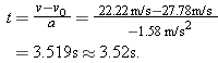(Answer)

If you are initially speeding and then try to slow to the speed limit, there is plenty of time for the police officer to measure your speed.

PROBLEM-SOLVING TACTICS

TACTIC 6: Check the Dimensions

To check the dimensions of Equation 2-15 (x - x₀ = v₀t + ½at²), note that every term must be a length, because that is the dimension of x and of x₀. The dimension of the term v₀t is (L/T)(T), which is L. The dimension of ½at² is (L/T²)(T²), which is also L. Thus, this equation checks out.

2.27 Interactive Learningware

20.29 Interactive Learningware

Copyright © 2000-2003 by John Wiley & Sons, Inc. or related companies. All rights reserved.