| 2-3 |
 |
|
Representing Motion Graphically |
When we plot position versus clock reading, the slope is
and therefore tells us the object's average velocity. Equation 2-6 has the standard form of a linear or straight line equation: v in Equation 2-6 has the same role as m in y = b + mx, the standard equation for a straight-line graph of y versus x.
 |
|
For WebLink 2-2: Proportionality, Rates, Slope, and Straight Lines and
|
To review basic ideas about linear equations and for more on how this math applies to real-world situations, go to WebLinks
2-2 and 2-3. Even if you are confident about the math, these WebLinks will help you think about the math in ways that are useful for
application to physics.
 Vertical Intercepts and their Meaning The vertically plotted variable is now x rather than y, so its initial value xo is the vertical intercept. The following example treats the graphing of a uniform motion situation in detail.
|
|
Example 2-3
|
|
Driving on Cruise Control |
|
|
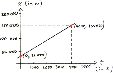
Cruise control keeps your car automatically at constant speed. An SI-oriented teenager has been heading east for 4000 s with
the cruise control set at 31 m/s (almost 70 miles/hour). He is now 150 000 m east of Ridgemont.
|
a.
|
How far east of Ridgemont did he start out?
|
|
|
b.
|
Sketch a graph of x versus t for this motion.
|
|
Brief Solution
|
a.
|
Assumptions.If we think of the instant he started out as t = 0, the given information then tells us that his position is x = 150 000 m at t = 4000 s.
|
|
Mathematical solution.
Solving for xo in Equation 2-6 gives us
|
b.
|
We need two points to determine a straight line. We now know x at two instants t because xo is by definition the value of x at t = 0. We can therefore plot the two points (t = 0, x = 26 000 m) and (t = 4000 s, x = 150 000 m) and draw the straight line connecting them. The resulting graph is shown at left.
|
|
|
 Related homework: Problems 2-18 and 2-19. Related homework: Problems 2-18 and 2-19. |
|
|
|
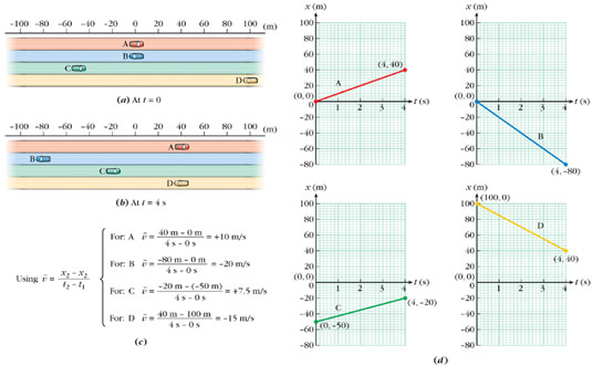
Interpreting Slope Positions and velocities, and also the slopes that represent velocities, may be either positive or negative. To reinforce
your understanding of how the signs work in various situations, consider Figure 2-6. Parts a and b show the positions of four cars at two different instants (t = 0 and t = 4 s). We shall assume that each car is being driven at uniform velocity. Note that when the cars are to the left of the
origin they have negative positions.
|
|
| Figure 2-6
Representations of uniform motion. We can use either pictures (a and b), equations (c), or graphs (d) to communicate aspects of the motion. As you come to understand them better, these different ways of representing the motion
should reinforce each other.
|
In Figure 2-6c, we use two positions x and the corresponding instants t to calculate the average velocity of each car. For each car, the two pairs of values give us two points on a plot of x versus t (Figure 2-6d). The two points determine the straight line graph for that car. Each average velocity in c is the slope of the corresponding graph in d. The graphs have constant slope—that's what makes them straight lines—because the cars are moving at constant velocity.
Let's see what some of the features of the graphs in d represent. (Note: If possible, you should try to explore these motions with a motion detector.)
|
|
|
|
Aspect of Motion Represented
|
|
|
|
|
|
|
The graphs for cars A and C slant upward to the right (their slopes are positive).
|
|
|
|
|
|
Cars A and C are moving toward the right. Their displacements as time advances are positive; thus, their velocities are positive.
|
|
|
|
|
|
The graphs for cars B and D slant downward to the right (their slopes are negative).
|
|
|
|
|
|
Cars B and D are moving toward the left, giving negative displacements and therefore negative velocities.
|
|
|
|
|
|
The graphs for cars B and C lie below the horizontal axis.
|
|
|
|
|
|
Cars B and C are to the left of the origin throughout the interval, so their positions x are always negative.
|
|
|
|
|
|
The graph for car C lies below the x axis, but the slope is positive.
|
|
|
|
|
|
C is positioned to the left of the origin during this interval but is moving toward the right.
|
|
|
|
|
|
The graph for car D lies above the x axis, but the slope is negative.
|
|
|
|
|
|
D is positioned to the right of the origin during this interval but is moving toward the left.
|
|
|
|
|
|
A's graph is steeper than C's (the scale is the same).
|
|
|
|
|
|
A is going at greater speed than C (also at greater velocity).
|
|
|
|
|
|
B's graph is steeper (more nearly vertical) than D's. Its slope is more negative, so the absolute value of its slope is greater.
|
|
|
|
|
|
B is going at greater speed than D (but not at greater velocity—a more negative number is not greater than a less negative number).
|
|
|
|
|
|
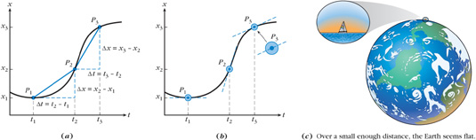
The idea of slope, a property of a straight line, can also be applied to nonuniform motion, such as the motion graphed in
Figure 2-7a. If you draw a straight line segment or secant connecting the points P1 and P2 on the graph, its slope is  , which is the average velocity v
. The straight line segment connecting points P2 and P3 has a greater slope, so the average velocity is greater over this interval. Interval by interval, the slopes of the straight
secants tell us about the motion represented by the curve.
, which is the average velocity v
. The straight line segment connecting points P2 and P3 has a greater slope, so the average velocity is greater over this interval. Interval by interval, the slopes of the straight
secants tell us about the motion represented by the curve.
|
|
| Figure 2-7
Interpreting slope for graphs of nonuniform motion.
|
If we want to know about instantaneous velocity, we can zoom in until we are looking at a segment of the curve that still
includes the instant in question, but is so tiny that it is essentially straight (Figure 2-7b). In the same way, as Figure 2-7c shows, a small stretch of ocean surface on a windless day may appear flat, even though the Earth is round. To help see how
the segments are sloping, we extend them (dotted in Figure 2-7b). Each extended line is very nearly a tangent, a line that just grazes the graph at a single point. So we can pick a tiny
close-up segment of the curve that includes a certain instant t, and we can take the slope of this segment to be a very good approximation to the instantaneous velocity at t. In other words, we find the instantaneous velocity approximately by applying Procedure 2-1 to this tiny segment.
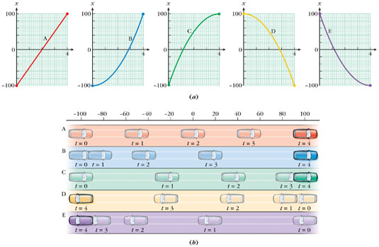
Graphs are a concise way of communicating a great deal of information about the motion of an object, whether uniform (constant
velocity) or not. It is therefore important for you to learn to read their features. WebLink 2-4 provides an opportunity to develop some experience with this. Figure 2-8 summarizes the motions treated in the WebLink and their graphs.
|
|
| Figure 2-8
(a) Graphs of position versus clock reading for cars with constant (A) and nonconstant (B–E) velocities. See WebLink 2-4 for more detail. (b) Picturing the motions described by these graphs. The centers of the cars are at the graphed positions.
|
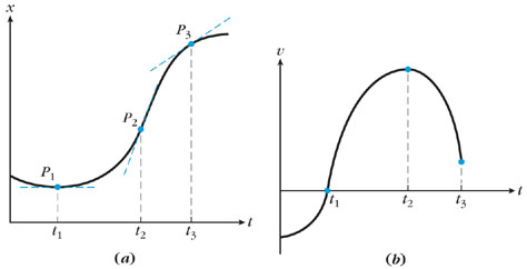
Graphs of v Versus t
We have already seen how to use the idea of slope to find the instantaneous velocity v at each instant t. Because we can find a value of v for each value of t, we can also graph v versus t. Figure 2-9a shows x versus t (from Figure 2-7a) and v versus t graphs for the same motion. In the following table, note how the features of the v versus t graph correspond to those of the x versus t graph.
|
|
| Figure 2-9
Graphs of x versus t and v versus t for the same nonuniform motion. (a) In the x versus t plot, the slopes of the tangents give the velocities. (b) In the v versus t plot, those slopes are plotted against t. Note that the horizontal tangent at t1 has zero slope.
|
|
|
Example 2-4
|
|
Sketching v versus t Graphs |
|
|
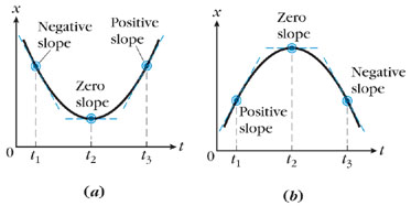
Figure 2-10 displays x versus t plots for two different moving objects. Sketch a graph of instantaneous velocity v versus clock reading t for each of these motions.
|
|
| Figure 2-10
x versus t graphs for two different moving objects.
|
Solution
Get the picture.
We first pick tiny segments of the curve at some typical values of t, because the slopes of these segments are roughly the instantaneous velocities at those values of t. This is done in Figure 2-11.
|
|
| Figure 2-11
The slopes of tiny segments of the graph give us the instantaneous velocities at different values of t.
|
See how v changes with t.
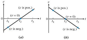
We see in Figure 2-11 that the slope of graph a is first negative (at t1), then zero (at t2), and then positive (at t3). Thus, the value of v goes from negative to zero to positive; like the slope that represents it, v is always increasing. The graph of v versus t must show v behaving in this way. The v versus t plot sketched in Figure 2-12a shows the required behavior.
|
|
| Figure 2-12
These graphs of velocity versus t are for the same motions as the x versus t graphs in Figures 2-10 and 2-11.
|
In contrast, the slope of graph b in Figure 2-11 is first positive (at t1), then zero (at t2), and then negative (at t3). The value of v likewise goes from positive to zero to negative; it is always decreasing. This behavior is displayed by the v versus t plot sketched in Figure 2-12b.*
|
Related homework: Problems 2-22, 2-23, and 2-24. |
|
|
|
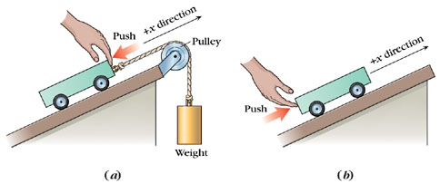
Figures 2-13a and 2-13b show real-world objects whose velocities behave in the manner described by the graphs in Figure 2-12 when set in motion by an initial push. You can see the graphs develop as the motions are animated in WebLink 2-5.
|
|
| Figure 2-13
These situations exhibit the motions that are graphed in Figures 2-10 through 2-12. In (a), the hand gives the car an initial velocity downhill. The net force on the car is uphill. In (b), the initial velocity is uphill, the net force downhill.
|
|
|
Copyright © 2004 by John Wiley & Sons, Inc. or related companies. All rights reserved.
|