| 2-5 |
|
Constant Acceleration and Equations of Motion |
![]() Constant Acceleration If an object's acceleration is constant, or uniform, its value never changes, so the instantaneous and average accelerations are the same. In that case, as in Figure 2-12, a graph of v versus t is a straight line, that is, its slope is the same everywhere.
Constant Acceleration If an object's acceleration is constant, or uniform, its value never changes, so the instantaneous and average accelerations are the same. In that case, as in Figure 2-12, a graph of v versus t is a straight line, that is, its slope is the same everywhere.
![]() Graphing Uniformly Accelerated Motion For constant acceleration, Equation 2-7 becomes
Graphing Uniformly Accelerated Motion For constant acceleration, Equation 2-7 becomes
 |
 gives us
 |
|
This has the general form y = b + mx or y = yo + mx of a straight line equation; t and v are the horizontally and vertically plotted variables, vo is the initial value of the latter—that is, the vertical intercept—and a is the rate of change or slope. To see how you can use this to interpret a graph of v versus t, let's work through Example 2-6.
|
|
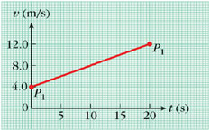
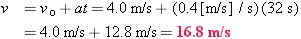
Interpreting a Linear Graph of v versus t | |||||||||||||||||||||||||||||
The velocity of a remote-controlled vehicle is plotted against time below.
Brief Solution Choice of approach. Note that v = vo + at has the same form as y = yo + mx.
|
||||||||||||||||||||||||||||||
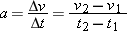
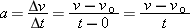
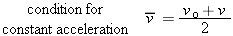
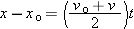
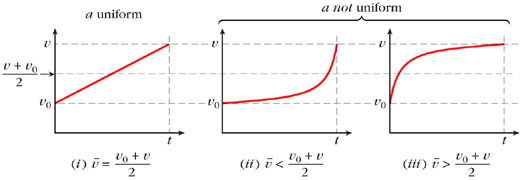
![]() Average Velocity Suppose an object accelerates uniformly from a velocity vo at t = 0 to a velocity v at some later instant t. The average velocity over this interval will then be midway between the values of vo and v. In other words, it is the numerical average of these two values:
Average Velocity Suppose an object accelerates uniformly from a velocity vo at t = 0 to a velocity v at some later instant t. The average velocity over this interval will then be midway between the values of vo and v. In other words, it is the numerical average of these two values:
 for most of the interval from 0 to t, so its time-averaged value is lower. For graph iii, by similar reasoning, the average velocity is higher than .
|
|||
| Figure 2-15 Average velocities for cases of uniform and nonuniform motion. |
Before solving problems about uniformly accelerated bodies, we should first ask where in the real world do we find bodies experiencing constant acceleration? We will have more to say about the conditions needed for constant acceleration in Chapters 4 and 5, when we discuss how objects affect one another's motions. For now, we won't try to generalize. We simply acknowledge that there is constant acceleration when measurements show that there is, and we give examples of this occurring.
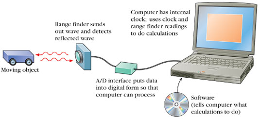
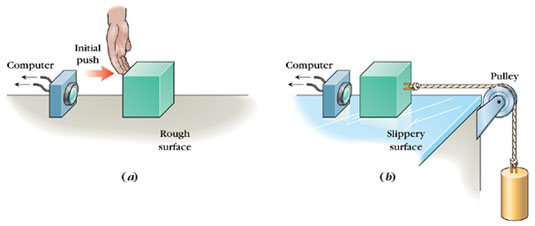
![]() Range Finder Measurements One way of doing the necessary measurements is with a sonic range finder (or motion detector) connected to a computer (Figure 2-16). Software loaded into the computer enables it to do calculations and plot graphs using the input from the range finder.
The range finder emits ultrasound pulses that travel at constant speed. It determines how far away a body is by sending out
a pulse, detecting the pulse reflected back from the body, and timing the duration of the round trip. One common model makes
15 such measurements each second, so that for a moving body, displacements Δx can be calculated for tiny intervals Δt, which are measured by the computer's internal clock. Then, using
Range Finder Measurements One way of doing the necessary measurements is with a sonic range finder (or motion detector) connected to a computer (Figure 2-16). Software loaded into the computer enables it to do calculations and plot graphs using the input from the range finder.
The range finder emits ultrasound pulses that travel at constant speed. It determines how far away a body is by sending out
a pulse, detecting the pulse reflected back from the body, and timing the duration of the round trip. One common model makes
15 such measurements each second, so that for a moving body, displacements Δx can be calculated for tiny intervals Δt, which are measured by the computer's internal clock. Then, using  , the software directs the computer to calculate values of average velocities that are approximately instantaneous because
the intervals are so small. From these values, the computer can therefore use
, the software directs the computer to calculate values of average velocities that are approximately instantaneous because
the intervals are so small. From these values, the computer can therefore use  to calculate acceleration values that are likewise approximately instantaneous. Using these simple equations (which do not require a to be uniform) to do hundreds of calculations each second, the computer can find x, v, and a at successive clock readings t, and it can display the results as graphs.
![]()
![]()
Figure 2-16
Range finder set-up for motion measurements.
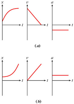
Figure 2-17 shows two situations for which these measurements are easily done. In 2-17a, the hand gives the block a shove to the right and the detector is turned on (t = 0) as soon as the block leaves the hand. In 2-17b, the detector is turned on when the weight strung over the pulley begins to fall. Figure 2-18 shows the resulting graphs. (Compare the x versus t plots with the graphs for cars B and C in Figure 2-8.) The v versus t graphs have constant slope, so the acceleration  is uniform. The a versus t plots reinforce this point: They are horizontal—the value of a is not going up or down.
|
|||
| Figure 2-17 Making measurements on the motion of a block with a range finder. |
|
|||
| Figure 2-18 Motion graphs for the blocks in Figure 2-17. |
Recall that the v versus t graphs (in Figure 2-12) for the carts in Figure 2-13 are also straight lines, so the carts' accelerations are also constant. In short, there are a variety of situations that we can treat as having constant or roughly constant acceleration.
|
|
A Racing Car Speeds Up | ||||||||||||||
|
A racing car goes from 30 m/s to 50 m/s over a 5.0-s interval. If the acceleration is constant, how far does it go during this time?
Solution Restating the problem. The question asks for a distance traveled during a time interval: What is |Δx| during a particular Δt of 5 s if v changes from v1 = 30 m/s to v2 = 50 m/s during this time interval? What we know/what we don't.
Choice of approach.
(1) Because the acceleration is constant, the average velocity meets the condition that The mathematical solution.
|
|||||||||||||||
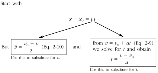
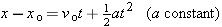
![]() Completely Describing Motion from Initial Conditions Suppose an object starts out at t = 0 with a certain initial velocity vo, and it has an acceleration a, which we know is constant. From the definition of acceleration, we obtained Equation 2-9, which can tell us the velocity v of the object at each subsequent instant t (see Example 2-6b). To describe the object's motion completely, we would need to know not only its velocity but its position x (or its displacement x − xo) at each instant. To find an expression that tells us this, we can reason algebraically from definitions and the condition
for constant acceleration.
Completely Describing Motion from Initial Conditions Suppose an object starts out at t = 0 with a certain initial velocity vo, and it has an acceleration a, which we know is constant. From the definition of acceleration, we obtained Equation 2-9, which can tell us the velocity v of the object at each subsequent instant t (see Example 2-6b). To describe the object's motion completely, we would need to know not only its velocity but its position x (or its displacement x − xo) at each instant. To find an expression that tells us this, we can reason algebraically from definitions and the condition
for constant acceleration.
The definition of average velocity (Equation 2-3) now becomes  , so that
 |
 (Equation 2-10), so
 |
 |
 |
|
Compare Equation 2-11 with x − xo = vt, which is valid whenever v is constant. If v does not change from its initial value vo, then a, its rate of change, is zero, and Equation 2-11 reduces to x − xo = vot. Otherwise, the last term on the right-hand side of Equation 2-11 represents an additional contribution to the position. This contribution is needed because the velocity is changing.
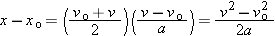
In describing a body's motion, you may also wish to find its velocity at each position x, without having to know t. To obtain an equation that does this, we start with what we already know and do some algebra:
|
 |
 |
|
Note that solving for v would then give you
 |
|
Copyright © 2004 by John Wiley & Sons, Inc. or related companies. All rights reserved. |


 to find Δ
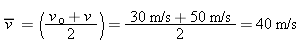
 .
.