| 2-2 |
 |
|
A Vocabulary for Describing Motion |
We often use terms like speed, distance, and time when describing motion. But even these terms are not sufficiently clear for our purposes. In ordinary language, for example,
we use the word time in two distinct ways. If I ask, “What time is it?,” you might reply “a quarter to two” or “9:54 AM.” If I ask, “How much time do you need?,” you might respond with something like “2 hours.” No proper response to the first question legitimately answers the second and vice versa; yet in both cases I am asking for
“the time.” We need to distinguish between specific instants or clock readings, on the one hand, and time intervals or durations on the other.
|
 |
|
|
For some of nature's creatures, one-dimensional motion comes naturally.
|
|
 Instants and Intervals If I ask you for an instant (“At what time … ?”), you need look at your watch only once to respond. If I ask you for a time interval (“How long does it take to do X?”), you must look at your watch twice, when you start and when you finish. If your readings were 3 o'clock and 5 o'clock, you
would then conclude that it took you 5 hr − 3 hr = 2 hr. We will denote an instant, a single clock or watch reading, by t. To find an interval, which we denote by Δt, we need to obtain two readings, t1 and t2, and subtract the earlier reading from the later one:
Instants and Intervals If I ask you for an instant (“At what time … ?”), you need look at your watch only once to respond. If I ask you for a time interval (“How long does it take to do X?”), you must look at your watch twice, when you start and when you finish. If your readings were 3 o'clock and 5 o'clock, you
would then conclude that it took you 5 hr − 3 hr = 2 hr. We will denote an instant, a single clock or watch reading, by t. To find an interval, which we denote by Δt, we need to obtain two readings, t1 and t2, and subtract the earlier reading from the later one:
The triple-bar equal sign tells you this is a definition.
Point Objects When an object moves, it changes its position during some time interval. If we are not careful, however, this claim can get
us into some silly discussions, such as:
We avoid all this by thinking first about an object small enough so that we can treat it mentally as though it were no more
than a point. We call such an object a point object or point particle.There is no such thing as a point object in nature. But it can be a useful way of thinking about a larger object when the
object's size doesn't matter. For example, in describing the motion of a car on a cross-country drive, the length of your
car is such a tiny fraction of the distance traveled that it might as well be a point. Physicists say its size is negligible in this situation. But if your car goes into a skid on an icy turn, you are very concerned that the tail of the car may be
moving differently than the front end; in that case, a point object approximation would cut out much of what is of interest
in analyzing the situation. We could, however, treat each tiny piece of the car as a separate point object. In that way, developing
a description of the motion of point objects lays a foundation for describing the motions of all objects. We will start by
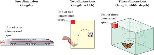
describing one-dimensional (straight-line) motion. We'll then extend our ideas to two-dimensional motion (Figure 2-1) in Chapter 3.
|
|
| Figure 2-1
Motion in one, two, and three dimensions.
|
Positions and Distances We can describe the position of any point or point object by giving its coordinates on some set of coordinate axes. Each axis is basically a real number
line. For one-dimensional motion, position means location along a single real number line, on which consecutive integers are
one unit (such as a meter) apart.
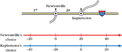
We can picture such a number line stretched along a long, straight road (Figure 2-2). But where should the zero go? The choice is yours; it depends on what question you wish to address. If you are interested
in how far things are from Newtonville in Figure 2-2, you would choose the red number line, with its zero fixed at Newtonville. If you care about distances from Keplertown, on
the other hand, the blue number line's zero is better located. Once we choose a particular number line, we can measure an
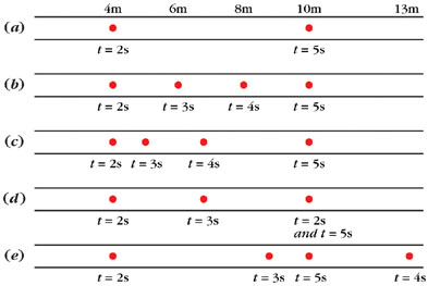
object's position at various instants during its motion. In Figure 2-3a, for example, the ball's position has been measured at t = 2 s and again at t = 5 s.  Based on these two measurements, what can we say about the total distance the ball traveled during that 3-s interval?

|
|
| Figure 2-2
Number lines or axes to indicate position.
|
|
|
| Figure 2-3
Different ways of achieving the same displacement and average velocity.
|
In fact, those two measurements provide no details about how the ball moved during the interval. Any of the scenarios shown
(Figures 2-3b to 2-3e) is possible; the number of possibilities is infinite. If (as in Figure 2-3e) the motion is not all in one direction, the total distance traveled is not just 10 m − 4 m = 6 m. Even in Figure 2-3b, we cannot say for certain that the ball traveled 6 m, because there might have been back-and-forth motion in between clock readings (say, between t = 3 s and t = 4 s). All we know for sure is that in each of the scenarios the net or resulting change in position was 6 m to the right during the 3-s interval depicted. We call this change in position the displacement Δx in one dimension:
The displacement tells you how far x2 is from x1, but not how far an object has traveled to get to x2 from x1. In contrast, distance is the length of the actual path traveled. Each piece of the overall length is positive, so the longer
you travel, the greater the distance you've gone.
Table 2-1 summarizes the relationships among these quantities and the type of question each quantity addresses.
| Table 2-1 Basic Quantities Used in Describing Motion |
|
|
|
|
|
|
|
|
|
|
|
|
Number line or coordinate axis reading, point in space
|
|
|
|
|
|
|
Clock reading, point in time
|
|
|
|
|
|
Time duration, time elapsed
|
|
|
|
|
|
|
|
|
|
|
|
|
|
|
How far … ? (and sign tells, Which way … ?)
|
|
|
|
|
|
When … ? At what time … ?
|
|
|
|
|
|
How long … ? How much time … ?
|
|
|
|
|
|
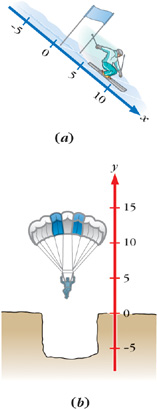
Notation A straight line path may be horizontal, diagonal, or vertical (Figure 2-4). If we use y instead of x for position along a vertical path, then the displacement between two points would be Δy = y2 − y1.
|
|
| Figure 2-4
Axes indicating position needn't be horizontal.
|
Negative Values When we use a real number line to identify position along a straight line, half of all possible positions will have negative
values. In Figure 2-2, a position 3 m to the left of the origin is expressed as x = − 3 m.
|
|
Example 2-1
|
|
Negative and Positive Displacements |
|
|
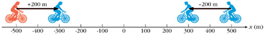
Find the displacement of a cyclist who rides
|
a.
|
from a position of 500 m to a position of 300 m.
|
|
|
b.
|
from a position of −500 m to a position of −300 m.
|
|
|
c.
|
Find the distance traveled by the cyclist in each case (assuming no backtracking).
|
|
Solution
Sketch the situation.
It is important to have a clear picture of what is happening. Figure 2-5 shows the displacements asked for in a and b.
|
|
| Figure 2-5
Positions and displacements for Example 2-1.
|
Use the definition.
Displacement is defined as Δx = x2 − x1, where x1 is the earlier and x2 the later position. In a, x1 = 500 m and x2 = 300 m, so
and is negative. In b, however, x1 = −500 m and x2 = −300 m, so
and is positive.
|
c.
|
The absolute value of either displacement is 200 m, so the distance traveled is 200 m in each case. Distances are always positive.
|
|
Making sense of the results.
In all cases,
|
if the motion is to the right along a left-to-right real number line, the displacement is positive and if it is to the left,
the displacement is negative.
|
|
|
Figure 2-5 illustrates this point.
|
 Related homework: Problems 2-7, 2-8, and 2-9. Related homework: Problems 2-7, 2-8, and 2-9. |
|
|
|
In one sense, the displacement provides more information than the distance: It answers not only “How far?” but “Which way?” as well. In the same spirit, we wish to address “How fast?” and “Which way?” together. To do so, we define a quantity v
called the average velocity during a time interval Δt (the bar over the v denotes average):
You can find the average velocity of an object using a meter stick and a clock. The definition is equivalent to the following
procedure:
| Procedure 2-1 |
|
|
| Determining Average Velocity in One Dimension |
|
|
1.
|
Measure the object's coordinate x1 at instant t1.
|
|
|
2.
|
Measure the object's coordinate x2 at instant t2 (later than t1).
|
|
|
3.
|
Calculate the increments Δx = x2 − x1 and Δt = t2 − t1.
|
|
|
4.
|
Divide Δx by Δt to obtain v
.
|
|
|
|
With t2 as the later instant, Δt is positive. Then v
has the same sign as the displacement Δx, and thus is in the same direction. We still need to clarify two aspects of average velocity: (1) why average? and (2) how is velocity different than our everyday notion of speed?
Why Average? Consider Figure 2-3. The ball in Figure 2-3a is at position x1 = 4 m when the clock reads t1 = 2 s and at x2 = 10 m when t2 = 5 s. The ball's displacement is therefore Δx = 10 m − 4 m = +6 m (to the right) during a time interval Δt = 5 s − 2 s = 3 s. During this time interval, the average velocity is  (also to the right). But Figure 2-3a provides no infor-mation about how the ball moved between the two instants t = 2 s and t = 5 s. The possible scenarios in Figures 2-3b to 2-3e show that the ball may have traveled at uniform speed, sped up, gotten to x = 10 m quickly and then stopped there until t = 5 s, and so on. We can't say which scenario the ball followed or how fast it was going at any particular instant during
the interval, only that its velocity averaged 2 m/s for the whole 3-s interval.
(also to the right). But Figure 2-3a provides no infor-mation about how the ball moved between the two instants t = 2 s and t = 5 s. The possible scenarios in Figures 2-3b to 2-3e show that the ball may have traveled at uniform speed, sped up, gotten to x = 10 m quickly and then stopped there until t = 5 s, and so on. We can't say which scenario the ball followed or how fast it was going at any particular instant during
the interval, only that its velocity averaged 2 m/s for the whole 3-s interval.
How is Average Velocity Different than Speed (or Average Speed)? Physicists are basically stating the everyday notion that most people have of speed when they define average speed as the total distance traveled divided by the time spent traveling:
 |
(2-4)
|
|
 |
|
|
An albatross gliding on prevailing winds. In the Southern Hemisphere, albatrosses have been known to go completely around the Earth in this way. At 40° south latitude, what information would you need to look up to calculate how long this trip would take?
|
|
For each segment with no direction reversals, the key difference is this: The average velocity can be positive or negative; the sign indicates its direction. The average speed is always positive; it provides no information about direction. When there are direction reversals, the average speed and average velocity can have numerically different values, as in
the following example.
|
|
Example 2-2
|
|
Average Speed versus Average Velocity |
|
|
For the motion of the ball in Figure 2-3e during the time interval from t = 2 s to t = 5 s, find a. the total distance, b. the total displacement, c. the average speed, and d. the average velocity. Assume the only change in direction occurs at t = 4 s.
Solution
Choice of approach.
We can find the average speed and average velocity from their definitions (Equations 2-4 and 2-3). Because distance equals |x2 − x1| only for path segments in which the object doesn't reverse direction, we must find separately the distances traveled from
t = 2 s to t = 4 s and from t = 4 s to t = 5 s, and then add the two distances. We will get the same displacement, however, whether we add the displacements for the
two shorter intervals or just subtract the position at t = 2 s from the position at t = 5 s.
The mathematical solution.
To make comparison easier, we will arrange the calculations in a table.
|
|
|
|
|
|
|
|
|
|
|
|
Between t = 2 s and t = 4 s
|
|
|
|
|
|
Between t = 4 s and t = 5 s
|
|
|
|
|
|
|
Between t = 2 s and t = 4 s
|
|
|
|
|
|
Between t = 4 s and t = 5 s
|
|
|
|
|
|
|
Between t = 2 s and t = 5 s
|
|
|
|
|
|
|
|
|
|
|
|
|
|
|
|
|
|
|
A critical feature of the calculations is that unlike the distance, the displacement from t = 4 s to t = 5 s is negative. This leads to an average velocity that is different than the average speed.
|
|
|
Instantaneous Velocity
To find an average velocity experimentally, you must take position readings at two instants. These measurements cannot tell
you how fast something is going at any single instant. If you want to know the velocity at a particular instant t, you must approach it by taking readings for smaller and smaller time intervals containing that instant. Using these measurements,
you find the average velocity for each interval. These average velocity values close in on a particular value (called a limiting value) as Δt shrinks closer and closer to zero (Δt → 0). To see in detail how this works, work through WebLink 2-1. This limiting value is what we call the instantaneous velocity at t.
The symbol v with no bar above it denotes instantaneous velocity. Just as average velocity only has meaning over a particular time interval, instantaneous velocity only has meaning at a
particular point in time—a particular instant t.
We've defined the average velocity as  . Suppose we choose the first instant t1 to be t = 0. This is like resetting our stopwatch to t = 0 when we start our observations. We can let xo denote the object's position at this instant, so that xo and 0 become the “values” of x1 and t1. If x represents its position at any later instant t (so that these become the “values” of x2 and t2), then
Solving for x in this equation gives us
 |
(2-6)
|
In words,
Both xo and v
t are lengths. Adding them gives a total length.
Uniform Motion When an object's velocity is uniform (the same at every instant during the time interval being analyzed), we do not have to distinguish between average velocity
v
and instantaneous velocity v. Then Equation 2-6 becomes
 |
(2-6a)
|
|
|
Copyright © 2004 by John Wiley & Sons, Inc. or related companies. All rights reserved.
|

 denotes “absolute value of Δx”; it is always positive.


 . Then, shrinking Δt to zero, we can take the absolute value of the instantaneous velocity to be the instantaneous speed.


 =
=  =
=