2-6	Solving Kinematics Problems I: Uniform Acceleration

We have begun doing kinematics, the mathematical description of motion. Equations 2-9, 2-11, and 2-12 are called the equations of motion or the kinematic equations for a uniformly accelerated body. They describe various aspects of the body's motion—for example, they tell where the object is at each instant, or what its velocity is at each position.

The first step in solving a problem in physics is to determine which physical principles and definitions are relevant to the problem, then let that guide your selection of equations. In kinematics problems, the most basic relationships are the definitions of average velocity and average acceleration. In addition, if the acceleration is uniform, we can write that the average velocity v is . Equations 2-9 to 2-12 follow algebraically from these more fundamental relationships. You cannot solve any problem with them that cannot be solved using the more fundamental relationships. Sometimes, in fact, it is easier to start from fundamentals (see Example 2-7). Other times, it may be more convenient to use the equations of motion.

	Example 2-8		Example 2-7 Revisited
	Repeat Example 2-7 using the equations of motion. Solution Restating the problem. Although the question asks for a distance traveled during a time interval, it is often convenient to assume that the object in question is starting out at x = 0 and t = 0. (This is just a matter of deciding where to put your origin and when to start your stopwatch.) With this assumption, Δx = x − xo = x − 0 = x and Δt = t − 0 = t. The question then becomes x = ? when t = 5 s. What we know/what we don't. Choice of approach. Because the acceleration a is unknown, we first solve Equation 2-9 for a. Once a is known, you can use Equation 2-11 to find x. The mathematical solution. Solving Equation 2-9 for a gives (Notice that this step is equivalent to using the definition of average acceleration.) Equation 2-11 then gives us  Related homework: Problem 2-38.

In general, we can use the kinematic equations to generate tables of numbers. With the numbers, we plot graphs. From the graphs, we “read” how the object moves. It is therefore very important for you to get used to reading and interpreting graphs. To see how the kinematic equations generate motion graphs for the ball in Figure 2-19a, work through Example 2-9.

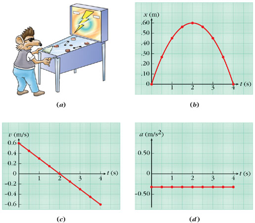
Figure 2-19  Describing a ball's motion graphically (see Web Example 2-9). (a) Dastardly Dude checks out the pinball machine by firing the ball gently enough so that it rolls uphill a short distance then returns to the plunger. The graphs that follow describe the ball's motion: (b) its position versus time, (c) its velocity versus time, and (d) its acceleration versus time.

	Example 2-9		Uniform Acceleration Pinball
	For a guided interactive solution, go to Web Example 2-9 at www.wiley.com/college/touger A pinball machine slopes slightly downward toward the player (Figure 2-19). Dastardly Dude, local pinball champ, gets the feel of the plunger by first shooting the ball gently enough so that it rolls back to the plunger. When he does so, the ball leaves the plunger with an initial velocity of 0.60 m/s. Its velocity 1.0 s later is 0.30 m/s. a.   Find the ball's acceleration. b.   Find its velocity every half second from t = 0 to t = 4 s. c.   Find its distance from the plunger every half second from t = 0 to t = 4 s. d.   Sketch graphs of x versus t, v versus t, and a versus t for the time period from t = 0 to t = 4 s. Brief Solution Restating the question. If xo = 0, then in part c we need only find x. What we know/what we don't. Choice of approach. When the acceleration is uniform, we can use the definition of average acceleration to find a. Once a is known, we can use Equation 2-9 to find v at other values of t and Equation 2-11 to find x at each value of t. Mathematical solution to parts a– c. The definition gives us Note that the velocity has decreased, so the acceleration is negative. For parts b and c we will do a sample calculation for t =1.5 s. We can do the same for each value of t and make a table of the results, then use the table entries as coordinates to plot points Sample calculation. When t = 1.5 s, and Graphing the Results. The resulting graphs are summarized in Figure 2-19 b–d. To obtain the a versus t graph, recall that a is uniform; its value is −0.30 (m/s)/s at every value of t.  Related homework: Problems 2-40 and 2-41.

 Asking Questions that Equations can Answer In Example 2-9 it was not sufficient to ask “what is the value of x (or v)?” Because the values were changing, we always had to ask, “what is the value of x at a particular value of t?” The equations we use are always relationships between two or more variables. For an equation to be useful in solving for the answer to a question, the question cannot simply be, “What is the value of some quantity Q₁?” (Q₁ = ?) It must have a more complete form, such as

(Form 2-1)

(In words: What is the value of Quantity 1 when Quantity 2 = a known value?)

or “ and so on?” When a question of Form 2-1 is not completely stated, you need to state the rest of it for yourself. You must do this even for questions like “how far does an object go?” or “how long does it take to get there?,” as in the following example.

	Example 2-10		“How Far …?”
	For a guided interactive solution, go to Web Example 2-9 at www.wiley.com/college/touger The hand in Figure 2-13a gives the cart an initial downhill shove. The cart leaves the hand with a speed of 3.0 m/s. While traveling downhill, it loses speed at a rate of 5 (m/s)/s. How far down the ramp does it go before coming back up? Restating the question. The speed is the absolute value of the velocity. The rate at which the velocity changes is the acceleration. If we take the downhill direction to be positive, v1 = 3.0 m/s but is decreasing, so the acceleration must be negative: a = −5.0 (m/s)/s or −5.0 m/s each second. The turnaround point is the position where v = 0. The question “how far?” is really asking: Δx = ? as v changes from v1 = 3.0 m/s to v2 = 0. Brief Solution 1 (reasoning from fundamentals) Choice of approach. Knowing both values of v, we can (1) find v and (2) find Δv. Knowing Δv, we can use the definition of acceleration to find Δt. Then, knowing v and Δt, we can use the definition of average velocity to find Δx. What we know/what we don't. The mathematical solution. Over the interval in question, the velocity changes by The average velocity Since when the acceleration is constant, we can solve for Δt: Now, because Brief Solution 2 (using equations of motion) The One-Step Solution. Solving for x in Equation 2-12 (with xo = 0) gives us The Two-Step Solution. From Equation 2-9, With this value of t, Equation 2-11 gives us  Related homework: Problem 2-42.

Note: For beginning students, it is usually more instructive to do solutions starting from fundamentals whenever possible, because it keeps you thinking more about the physics (what is happening and what the various quantities mean) than about the algebra.

Copyright © 2004 by John Wiley & Sons, Inc. or related companies. All rights reserved.