|
Velocity |
 |
We use vectors not only to describe the position of an object but also to describe velocity (speed and direction). If we know
an object's present speed in meters per second and the object's direction of motion, we can predict where it will be a short
time into the future. As we have seen, change of velocity is an indication of interaction. We need to be able to work with velocities of objects in 3D, so we need to learn
how to use 3D vectors to represent velocities. After learning how to describe velocity in 3D, we will also learn how to describe
change of velocity, which is related to interactions.
Average Speed
The concept of speed is a familiar one. Speed is a single number, so it is a scalar quantity (speed is the magnitude of velocity).
A world-class sprinter can run 100 meters in 10 seconds. We say the sprinter's average speed is (100 m)/(10 s) = 10 m/s. In
SI units speed is measured in meters per second, abbreviated “m/s.”
A car that travels 100 miles in 2 hours has an average speed of (100 mi)/(2 hr) = 50 miles per hour (about 22 m/s). In symbols,
where
vavg is the “average speed, ”
d is the distance the car has traveled, and
t is the elapsed time.
There are other useful versions of the basic relationship among average speed, distance, and time. For example,
expresses the fact that if you run 5 m/s for 7 seconds you go 35 meters. Or you can use
to calculate that to go 3000 miles in an airplane that flies at 600 miles per hour will take 5 hours.
Units
While it is easy to make a mistake in one of the formulas relating speed, time interval, and change in position, it is also
easy to catch such a mistake by looking at the units. If you had written

, you would discover that the right-hand side has units of (m/s)/m, or 1/s, not s. Always check units!
Instantaneous Speed Compared to Average Speed
If a car went 70 miles per hour for the first hour and 30 miles an hour for the second hour, it would still go 100 miles in
2 hours, with an average speed of 50 miles per hour. Note that during this 2-hour interval, the car was almost never actually
traveling at its average speed of 50 miles per hour.
To find the “instantaneous” speed—the speed of the car at a particular instant—we should observe the short distance the car
goes in a very short time, such as a hundredth of a second: If the car moves 0.3 meters in 0.01 s, its instantaneous speed
is 30 meters per second.
Vector Velocity
Earlier we calculated vector differences between two different objects. The vector difference

represented a
relative position vector—the position of object 2 relative to object 1 at a particular time. Now we will be concerned with the change
of position of
one object during a time interval, and

will represent the “displacement” of this single object during the time interval, where

is the initial 3D position and

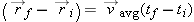
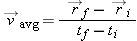
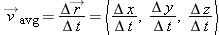
is the final 3D position (note that as with relative position vectors, we always calculate “final minus initial”). Dividing
the (vector) displacement by the (scalar) time interval
tf −
ti (final time minus initial time) gives the average (vector) velocity of the object:
Determining Average Velocity from Change in Position
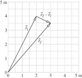
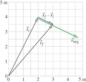
Consider a bee in flight (Figure
1.31). At time
ti = 15 s after 9:00
AM, the bee's position vector was
. At time
tf = 15.1 s after 9:00
AM, the bee's position vector was
. On the diagram, we draw and label the vectors
and
.
|
|
|
|
|

|
Figure 1.31 |
The displacement vector points from initial position to final position.
|
|
|
|
|
Next, on the diagram, we draw and label the vector
, with the tail of the vector at the bee's initial position. One useful way to think about this graphically is to ask yourself
what vector needs to be added to the initial vector

to make the final vector
, since
can be written in the form
.
The vector we just drew, the change in position
, is called the “displacement” of the bee during this time interval. This displacement vector points from the initial position
to the final position, and we always calculate displacement as “final minus initial.”
|
|
 Note that the displacement refers to the positions of one object (the bee) at two different times, not the position of one object relative to a second object at one particular time. However, the vector subtraction is the same
kind of operation for either kind of situation.
|
|
|
We calculate the bee's displacement vector numerically by taking the difference of the two vectors, final minus initial:
This numerical result should be consistent with our graphical construction. Look at the components of
in Figure
1.31. Do you see that this vector has an
x component of +1 and a
y component of −0.5 m? Note that the (vector) displacement
is in the direction of the bee's motion.
The average velocity of the bee, a vector quantity, is the (vector) displacement
divided by the (scalar) time interval
t f −
t i. Calculate the bee's average velocity:
Since we divided
by a scalar (
t f −
t i), the average velocity

points in the direction of the bee's motion, if the bee flew in a straight line.
What is the speed of the bee?
What is the direction of the bee's motion, expressed as a unit vector?
Note that the “m/s” units cancel; the result is dimensionless. We can check that this really is a unit vector:
This is not quite 1.0 due to rounding the velocity coordinates and speed to three significant figures.
Put the pieces back together and see what we get. The original vector factors into the product of the magnitude times the
unit vector:
This is the same as the original vector

.
| 1.X.29 |
At a time 0.2 seconds after it has been hit by a tennis racket, a tennis ball is located at  5, 7, 2  m, relative to an origin in one corner of a tennis court. At a time 0.7 seconds after being hit, the ball is located at 9, 2, 8 m.
|
|
(a)
|
What is the average velocity of the tennis ball?
|
|
|
(b)
|
What is the average speed of the tennis ball?
|
|
|
(c)
|
What is the unit vector in the direction of the ball's velocity?
|
|
|
|
|
|
|
| 1.X.30 |
A spacecraft is observed to be at a location 200, 300, −400 m relative to an origin located on a nearby asteroid, and 5 seconds later is observed at location 325, 25, −550 m.
|
|
(a)
|
What is the average velocity of the spacecraft?
|
|
|
(b)
|
What is the average speed of the spacecraft?
|
|
|
(c)
|
What is the unit vector in the direction of the spacecraft's velocity?
|
|
|
|
|
|
|
|
|
|
|
Scaling a Vector to Fit on a Graph
Moreover, the magnitude of the vector, 11.18 m/s, doesn't fit on a graph that is only 5 units wide (in meters). It is standard
practice in such situations to scale down the arrow representing the vector to fit on the graph, preserving the correct direction.
In Figure
1.32 we've scaled down the velocity vector by about a factor of 3 to make the arrow fit on the graph. Of course if there is more
than one velocity vector we use the same scale factor for all the velocity vectors. The same kind of scaling is used with
other physical quantities that are vectors, such as force and momentum, which we will encounter later.
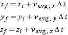
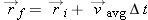
Predicting a New Position
We can rewrite the velocity relationship in the form
That is, the (vector) displacement of an object is its average (vector) velocity times the time interval. This is just the
vector version of the simple notion that if you run at a speed of 7 m/s for 5 s you move a distance of (7 m/s)(5 s) = 35 m,
or that a car going 50 miles per hour for 2 hours goes (50 mi/hr)(2 hr) = 100 miles.
Using the Position Update Formula
The position update formula
is a vector equation, so we can write out its full component form:
Because the
x component on the left of the equation must equal the
x component on the right (and similarly for the
y and
z components), this compact vector equation represents three separate component equations:
|
|
|
|
Updating the Position of a Ball
At time ti = 12.18 s after 1:30 PM a ball's position vector is  . The ball's velocity at that moment is 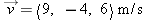 . At time tf = 12.21 s after 1:30 PM, where is the ball, assuming that its velocity hardly changes during this short time interval?
|
|
|
|
|
|
|
|
| 1.X.31 |
A proton traveling with a velocity of 3 × 10 5, 2 × 10 5, −4 × 10 5 m/s passes the origin at a time 9.0 seconds after a proton detector is turned on. Assuming that the velocity of the proton
does not change, what will its position be at time 9.7 seconds?
|
|
|
|
|
| 1.X.32 |
How long does it take a baseball with velocity 30, 20, 25 m/s to travel from location 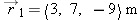 to location 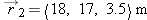 ?
|
|
|
|
|
|
|
|
|
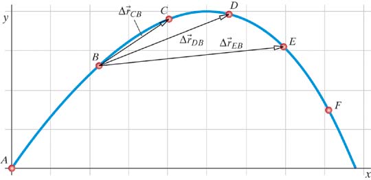
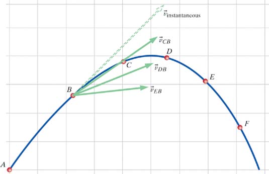
Instantaneous Velocity
Suppose we ask: What is the velocity of the ball at the precise instant that it reaches location B? This quantity would be called the “instantaneous velocity” of the ball. We can start by approximating the instantaneous
velocity of the ball by finding its average velocity over some larger time interval.
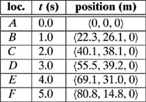
The table in Figure
1.34 shows the time and the position of the ball for each location marked by a colored dot in Figure
1.33. We can use these data to calculate the average velocity of the ball over three different intervals, by finding the ball's
displacement during each interval, and dividing by the appropriate Δ
t for that interval:
|
|
|
|
|
|
|
Figure 1.34 |
Table showing elapsed time and position of the ball at each location marked by a dot in Figure 1.33.
|
|
|
|
|
Simply by looking at the diagram, we can tell that

is closest to the actual instantaneous velocity of the ball at location
B, because its direction is closest to the direction in which the ball is actually traveling. Because the direction of the
instantaneous velocity is the direction in which the ball is moving at a particular instant, the instantaneous velocity is
tangent to the ball's path. Of the three average velocity vectors we calculated,
best approximates a tangent to the path of the ball. Evidently
, the velocity calculated with the shortest time interval,
t C −
t B, is the best approximation to the instantaneous velocity at location
B. If we used even smaller values of Δ
t in our calculation of average velocity, such as 0.1 second, or 0.01 second, or 0.001 second, we would presumably have better
and better estimates of the actual instantaneous velocity of the object at the instant when it passes location
B.
Two important ideas have emerged from this discussion:
|
|
|
The direction of the instantaneous velocity of an object is tangent to the path of the object's motion.
|
|
|
|
Smaller time intervals yield more accurate estimates of instantaneous velocity.
|
|
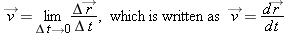
Connection to Calculus
You may already have learned about derivatives in calculus. The instantaneous velocity is a derivative, the limit of

as the time interval Δ
t used in the calculation gets closer and closer to zero:
In Figure
1.35, the process of taking the limit is illustrated graphically. As smaller values of Δ
t are used in the calculation, the average velocity vectors approach the limiting value: the actual instantaneous velocity.
A useful way to see the meaning of the derivative of a vector is to consider the components:
The derivative of the position vector

gives components that are the components of the velocity, as we should expect.
Informally, you can think of

as a very small (“infinitesimal”) displacement, and
dt as a very small (“infinitesimal”) time interval. It is as though we had continued the process illustrated in Figure
1.35 to smaller and smaller time intervals, down to an extremely tiny time interval
dt with a correspondingly tiny displacement
. The ratio of these tiny quantities is the instantaneous velocity.
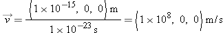
The ratio of these two tiny quantities need not be small. For example, suppose that an object moves in the
x direction a tiny distance of 1 × 10
−15 m, the radius of a proton, in a very short time interval of 1 × 10
−23 s:
which is one-third the speed of light (3 × 10
8 m/s)!
Acceleration
Velocity is the time rate of change of position:

. Similarly, we define “acceleration” as the time rate of change of velocity:

. Acceleration, which is itself a vector quantity, has units of meters per second per second, written as m/s/s or m/s
2.
If a car traveling in a straight line speeds up from 20 m/s to 26 m/s in 3 seconds, we say that the magnitude of the acceleration
is (26 − 20)/3 = 2 m/s/s. If you drop a rock, its speed increases 9.8 m/s every second, so its acceleration is 9.8 m/s/s,
as long as air resistance is negligible.
| 1.X.36 |
Suppose the position of an object at time t is 3 + 5 t, 4 t2, 2 t − 6 t3. What is the instantaneous velocity at time t? What is the acceleration at time t? What is the instantaneous velocity at time t = 0? What is the acceleration at time t = 0?
|
|
|
|
|
|
|
|
|
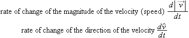
Change of Magnitude and/or Change in Direction
There are two parts to the acceleration, the time rate of change of the velocity

:
As we'll see in later chapters, these two parts of the acceleration are associated with pushing or pulling parallel to the
motion (changing the speed) or perpendicular to the motion (changing the direction).
|
| Copyright © 2011 John Wiley & Sons, Inc. All rights reserved. |