|
Potential Difference in a Nonuniform Field |
 |
Two Adjacent Regions with Different Fields
In the previous sections we considered only situations in which the electric field is uniform within a region. However, often
the real world is more complex than this. We need to be able to calculate changes in electric potential and electric potential
energy in regions of space in which the electric field is not uniform.
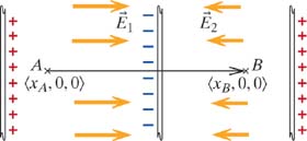
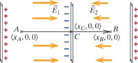
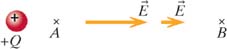
Consider a situation in which the path from the initial location to the final location of interest passes through two regions
of uniform but different electric field. In region 1 the electric field is

, and in region 2 the electric field is

, as shown in Figure
17.16. What would be the change in electric potential energy of a particle traveling along a path from location
A to location
B? (Assume that there is a tiny hole in the middle plate, so a particle can pass through it.)
|
|
|
|
|

|
Figure 17.16 |
The path from location A to location B passes through two regions in which the field is different.
|
|
|
|
|
In order to calculate Δ
V in this situation, we need to divide the path into two pieces. Each displacement vector

must be small enough that the electric field is uniform in the region through which it passes. Essentially, we have to invent
a new point, which we can call
C, on the boundary between the two regions, as shown in Figure
17.17.
|
|
|
|
|
|
|
Figure 17.17 |
We divide the path into two segments by inventing a point C. Each segment of the path now passes through a region of uniform electric field.
|
|
|
|
|
Now we can calculate the difference in potential along the two segments of the path:
|
From location A to location C:  |
|
From location C to location B:  |
|
From location A to location B:
|
|
In general, we need to add up all components (
x,
y, and
z), so we can write the general equation as a sum:
|
 |
|
Potential Difference Across Several Regions |
|
 |
|
|
|
 |
|
 |
|
|
|
|
|
Potential Difference Across Two Regions
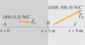
Suppose that from x = 0 to x = 3 the electric field is uniform and given by  , and that from x = 3 to x = 5 the electric field is uniform and given by  (see Figure 17.18). What is the potential difference Δ V = VC − VA?
|
|
|
|
|
|
|
Figure 17.18 |
The electric field differs in the two regions.
|
|
|
|
|
|
|
|
|
|
|
|
|
Split the path into two parts, A to B and B to C. In each part the electric field is constant in magnitude and direction. We have the following:
|
|
|
|
|
|
| 17.X.10 |
In the earlier Figure 17.17, location A is at  0.5, 0, 0  m, location C is 1.3, 0, 0 m, and location B is 1.7, 0, 0 m.  and  . Calculate the following quantities:
|
|
(a)
|
ΔV along a path going from A to B, and
|
|
|
(b)
|
ΔV along a path going from B to A.
|
|
|
|
|
|
|
|
|
|
|
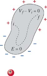
A Conductor in Equilibrium
In a conductor in equilibrium the difference in potential between any two locations is zero, because
E = 0 inside the conductor.
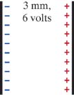
The direction of the electric field in the gap is toward the left, away from the positive plate and toward the negative plate.
The magnitude can be found from noting that the potential difference ΔV = Es = 6 volts, so that E = (6 volts)/(0.003 m) = 2000 volts/meter.
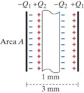
Does Inserting a Metal Slab Change ΔV? Next we insert into the center of the gap a 1-mm-thick metal slab with the same area as the capacitor plates, as shown in
Figure 17.21. We are careful not to touch the charged capacitor plates as we insert the metal slab. We want to calculate the new potential
difference between the two outer plates.
|
|
|
|
|
|
|
Figure 17.21 |
Insert a metal slab in the middle of the capacitor gap.
|
|
|
|
|
First we need to understand the new pattern of electric field that comes about when the metal slab is inserted. The charges
on the outer plates are −
Q1 and +
Q1, both distributed approximately uniformly over a large plate area
A. The metal slab of course polarizes and has charges of +
Q2 and −
Q2 on its surfaces, as indicated in Figure
17.21.
The electric field inside a capacitor is approximately
E = (
Q/A)/ε
0, where
Q is the charge on one plate and
A is the area of the plate, if the plate separation
s is small compared to the size of the plates.
The plates and the surfaces of the slab have the same area A. The outer charges −Q1 and +Q1 produce an electric field in the metal slab E1 = (Q1/A)/ε0 to the left. The inner charges +Q2 and −Q2 are arranged like the charges on a capacitor, so they produce an electric field in the metal slab E2 = (Q2/A)/ε0 to the right. The sum of these two contributions must be zero, because the electric field inside a metal in equilibrium must
be zero. Hence Q2 is equal to Q1.
As a result, the left pair of charges produces a field like that of a capacitor, and the right pair of charges also produces
a field like that of a capacitor. The effect is that after inserting the metal slab, the electric field is still approximately
2000 V/m in the air gaps but is now zero inside the metal slab. (The fringe fields are small if the gap is small.)
The electric field in the air gap is essentially unchanged, so
Δ
V inside the metal slab must be zero, because
E = 0 inside the slab. The potential difference between the plates of the capacitor is now:
not 6 V as it was originally. (Note that there is no such thing as “conservation of potential”; the potential difference changed
when we inserted the slab.)
A Powerful Reasoning Tool. When you know that the electric field inside a metal must be zero, you know that the sum of all the contributions to that
electric field must be zero. This is a powerful tool for reasoning about fields and charges in and on metals in equilibrium.
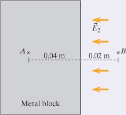
| 17.X.12 |
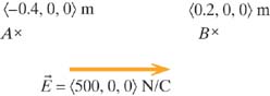
In Figure 17.22, location A is inside a charged metal block, and location B is outside the block. The metal block sits on an insulating surface and is not in contact with any other object. The electric
field outside the block is  .
|
|
|
|
|
|
|
Figure 17.22 |
Location A is inside a charged metal block. Location B is outside the block.
|
|
|
|
|
|
|
(a)
|
Calculate ΔV along a path going from A to B.
|
|
|
(b)
|
Calculate ΔV along a path going from B to A.
|
|
|
|
|
|
|
|
|
|
|
A Region of Varying Electric Field Requires an Integral
In some situations, the electric field in a region varies continuously. For example, the electric field due to a single point
charge is different in magnitude and direction at every location in space. To find a change in electric potential between
two locations in such a region, we need to take into account the varying electric field.
A Complete Procedure for Calculating Potential Difference
To calculate the potential difference between points
a and
b, always begin by considering the equation
|
|
(a)
|
Decide whether  varies in the region of interest. Draw the pattern of electric field throughout this region, making sure that you are considering
the electric field not only at points a and b, but at locations in space around those points as well.
|
|
|
(b)
|
Specify the origin and a set of axes for this situation.
|
|
|
(c)
|
Write as a function of position using the coordinates specified by your chosen axes.
|
|
|
(d)
|
Draw a path that connects points a and b. Be sure that your path starts at the initial location and ends at the final location. Based on this path and the electric
field in the region, predict the sign for the potential difference associated with moving along the path.
|
|
|
(e)
|
Convert  to a quantity that represents a displacement along the path you have chosen in the coordinates given by the axes.
|
|
|
(f)
|
Evaluate  and integrate (or sum numerically). Check the sign that you obtain after performing your integration and compare it against
your prediction.
|
|
Hints and Rules of Thumb
Remember that you are free to choose any path that connects the two points, since the electric potential difference between
two locations in space is independent of path.
Picking a path that takes into consideration the dot product

and the field pattern you've already drawn could significantly simplify the problem.
Potential Difference Near a Point Charge
We'll apply this procedure in a familiar situation: a region near a single point charge, as shown in Figure
17.23.
|
|
|
|
|
|
|
Figure 17.23 |
The electric field varies continuously along a path near a point charge.
|
|
|
|
|
|
|
(a)
|
In our drawing of the region around the point charge (Figure 17.23) we see that varies, so we need to use an integral.
|
|
|
(b)
|
We pick the location of the charge as the origin, with the x axis in the direction from location A to location B.
|
|
|
(c)
|
We write the field between A and B as a function of x:
|
|
|
(d)
|
We choose as our path a straight line along our x axis, from A to B. Since the direction of the path from A to B is the same as the direction of the electric field in the region, the potential difference should be negative.
|
|
|
(e)
|
We divide the path up into a very large number of infinitesimal steps, each of the same magnitude and direction. Instead of
, we will call each in-finitesimal displacement vector  .
|
|
|
(f)
|
|
|
The value of
x at location A is
xa, and the value of
x at location B is
xb, so these are the limits of integration:
We can determine the sign of this quantity by looking at both the sign of
Q and the difference

. In this case
Q > 0 and
xb > xa, so
is negative, and Δ
V is negative, as we expected in step (d).
If the point charge were negative, the potential difference would be positive; this also makes sense, since the electric field
would be opposite to the direction of the path.
|
|
|
|
Potential Difference Due to a Proton
A proton is located at the origin. Location C is 1 × 10 −10 m from the proton, and location D is 2 × 10 −8 m from the proton, along a line radially outward.
|
|
(a)
|
What is the potential difference VD − VC ?
|
|
|
(b)
|
How much work would be required to move an electron from location C to location D?
|
|
|
|
|
|
|
|
|
|
|
|
(a)
|
|
|
|
(b)
|
Work to move an electron: The least amount of work will be required if we don't change the kinetic energy of the proton.
|
|
|
|
|
|
|
|
General Definition of Potential Difference
This general expression is correct for regions in which the field is uniform, as well as for regions in which the field varies.
For example, in the situation shown in Figure
17.24, where the field is uniform,
The result of the integration is the same as we got in the example involving uniform field in Section
17.3.
|
|
|
|
|
|
|
Figure 17.24 |
A region of uniform electric field.
|
|
|
|
|
Limit on Mathematical Complexity in This Text
To establish the basic principles we will typically consider relatively simple situations. Often the electric field is uniform
(same magnitude and direction) all along a straight path, which makes the calculation very simple. Another relatively simple
situation is one in which the magnitude varies but not the direction along a straight path. A third simple situation that
we will encounter is one in which we move along a curved path, but the electric field is always in the same direction as this
curved path, and often constant in magnitude, which occurs in electric circuits. In each of these simple cases it can be quite
easy to evaluate the potential difference, as we saw in the preceding exercises.
|
|
|
|
|
|
|
|
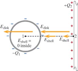
Final location: 2
This allows us to find ΔV due to the shell and ΔV due to the disk separately, then add them.
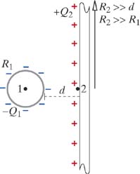
Simplifying assumption: Neglect the polarization of the plastic and glass, because there is little matter in the thin shell
and thin disk, so the field of the polarized molecules is negligible compared to the contributions of −Q1 and +Q2.
ΔV due to shell: Put origin at center of shell.
Inside the shell: Vsurface of shell − V1 = 0 because Eshell = 0 inside the shell.
To the right of the shell:
Check sign: As we move toward the disk, we're moving opposite to the field, so the potential should increase. Result agrees,
since +Q1/R1 is the larger term.
Δ V due to disk: an approximation is that since  and  ,
We could set up an integral, placing the origin at the center of the disk. However, since  is approximately uniform, we recognize that the result of integrating will be
Check sign: As we move toward the disk, we're moving opposite to the field, so the potential should increase. Result agrees.
Δ V due to both shell and disk:
|
|
|
|
|
|
|
|
|
| Copyright © 2011 John Wiley & Sons, Inc. All rights reserved. |


 to calculate the potential difference along a path that is not straight, such as that shown in Figure 17.25, along which the electric field is varying in magnitude and direction, can be mathematically challenging. In many cases the
best way to do this is to do it numerically, using a computer. In this text we will not ask you to do arbitrarily complex
integrations of this kind analytically.
to calculate the potential difference along a path that is not straight, such as that shown in Figure 17.25, along which the electric field is varying in magnitude and direction, can be mathematically challenging. In many cases the
best way to do this is to do it numerically, using a computer. In this text we will not ask you to do arbitrarily complex
integrations of this kind analytically.


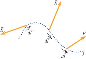
 . The potential difference
  is the sum of all these contributions.
 along a path from 1 to 2.
 according to the Superposition Principle, so